Introduction
In recent years, deep learning has required an increasing number of computationally heavy calculations, making the acceleration of deep learning workloads an important area of research. While most deep learning applications today use 32 bits of floating-point (FP) precision, various researchers have demonstrated the successful use of lower numerical precision in deep learning training and inference workloads.
The 2nd Generation Intel® Xeon® Scalable processor includes new embedded acceleration instructions known as Intel® Deep Learning Boost (Intel® DL Boost) that uses Vector Neural Network Instructions (VNNI) to accelerate low precision performance.
Read this tutorial to learn how to use the new Intel DL Boost accelerator on an inference workload. We provide a set of guidelines for running inference with both 32-bit FP precision and 8-bit integer precision using the Intel® Distribution of OpenVINO™ toolkit. For more information, see the Intel white paper Lower Numerical Precision Deep Learning Inference. We use a pre-trained model to guide you through the following processes:
- Transform a frozen graph into an intermediate representation (.bin or .xml), which is required by the Intel Distribution of OpenVINO toolkit.
- Run inference on the trained model (FP32) over our dataset, which is a 37-category set of pet images with roughly 200 images for each class. We show the accuracy of our model on the entire dataset and measure inference frames per second.
- Use the Calibration Tool (part of the OpenVINO™ toolkit) to quantize the model to INT8.
- Rerun the same inference application on the same dataset and same machine.
Finally, we compare the inference results of the FP32 and INT8 models.
Prerequisites
This tutorial was created using version 2019 R3.1 of the Intel Distribution of OpenVINO toolkit installed on a 2nd generation Intel Xeon Scalable processor.
Inference Flow with the Intel® Distribution of OpenVINO™ Toolkit
In an end-to-end deep learning development cycle where you have a well-trained model, after you have tuned parameters you need tools to deploy the model on the hardware of your choice. This is where the Intel Distribution of OpenVINO toolkit enters the picture. It quickly deploys applications and solutions that emulate human vision. The toolkit also maximizes performance for computer-vision workloads across Intel® hardware. It includes the Deep Learning Deployment Toolkit (DLDT), Open Model Zoo, Intel® Media SDK, and drivers and runtimes for OpenCL™, OpenCV, and OpenVX*.

Figure 1. Intel® Distribution of OpenVINO™ Toolkit inference flow
Using the deep learning Model Optimizer and deep learning inference engine, which are both part of the DLDT, we built an inference flow as shown in Figure 1. To start the process we made sure that our pre-trained model was in the correct format for conversion into an intermediate representation (IR). In this example, we start from Keras or TensorFlow*, which requires us to freeze our graph into the protobuf format to allow the deep learning Model Optimizer to read and convert it into an IR. See Supported Frameworks and Formats in Intel Distribution of OpenVINO toolkit for further details.
Next, we use the inference engine API to load plugins and the network parameters. After configuring the input and output files, we load our model parameters into the network, perform pre-processing to prepare our dataset, and call into the inference engine, which generates our model’s output.
While Figure 1 summarizes the flow of the inference model in this article, the Intel Distribution of OpenVINO toolkit offers several inference engine demos and inference engine samples to help you get started with a variety of models and workloads.
FP32 Model Inference Stages
This section explains the steps required to run FP32 inference:
- Create an IR (.bin or .xml) using the deep learning Model Optimizer.
- Understand the OpenVINO arguments.
- Instantiate the OpenVINO network.
- Run inference over a dataset.
Create the Intermediate Representation (IR)
Model Optimizer is a cross-platform command-line tool that facilitates the transition between the training and deployment environment, performs static model analysis, and adjusts deep learning models for optimal execution on end-point target devices.
Model Optimizer process assumes you have a network model trained using a supported deep learning framework. Figure 2 below illustrates the typical workflow for converting a trained model to an IR file using the OpenVINO Model Optimizer tool.

Figure 2. OpenVINO Model Optimizer flow
- Call out directly to the command line and look for the mo.py file.
- Add parameters for the input model and input shape of the topology. The command below generates the FP32 model of the IR by default. To generate the FP16 version, you must add --data_type=FP16 to the parameters.
mo.py --input_model=all_layers.rn50.pb --input_shape=[128,224,224,3] --mean_values=[123,117,104] --reverse_input_channels
For more details on this process, see Converting a Model to Intermediate Representation.
Instantiate the Network
Note: To review the specific steps for instantiating the network, see the inference.py file included in the Intel® IoT Developer Kit samples.
The general steps are as follows:
- Examine the parameters that were passed to the constructor. As shown below, you can see that the .XML file is passed as the base model, there are no CPU extensions, and the CPU is targeted as the device type.
- Call out to the constructor for the network instantiation.
- Load the model into that network by passing in the .bin and .xml parameters.
- Read in the labels file that you will use to decode the results during your inference.
from inference import Network
import warnings
warnings.filterwarnings("ignore")

arg_model="pets.rn50.xml"
arg_device="CPU"

# Initialise the class
infer_network = Network()
# Load the network to IE Core to get shape of input layer
infer_network.load_model(arg_model, arg_device, 1, 1, 2, None)
print("Network Loaded")

#Read in Labels
arg_labels="pets/pets-labels.txt"
label_file = open(arg_labels, "r")
labels = label_file.read().split('\n')
print("Labels Read")
Run the Inference
The code below shows the following six steps:
- Instantiate a figure to graph the output.
- Gather paths for images.
- Read the image and transform/preprocess.
- Start the inference request.
- Calculate the inference frames per second (FPS) and label.
- Update the graph every N steps.
import random
import glob
import os
from keras.applications.resnet50  import preprocess_input
from keras.preprocessing import image
from multiprocessing import Pool
import numpy as np
import tqdm
import math
import time

import matplotlib.pyplot as plt
%matplotlib widget
plt.rcParams.update({'font.size': 16})
from IPython.display import display, clear_output


file_list = glob.glob("pets/pets_images/*/*")
random.shuffle(file_list)

def process_images(img_path):
    img_cat = os.path.split(os.path.dirname(img_path))[1]
    img = image.load_img(img_path, target_size=(224, 224))
    img = image.img_to_array(img)
    img = np.transpose(img, (2, 0, 1))
    img = preprocess_input(img)
    return (img, img_cat)

if __name__ == '__main__':
	    print("Processing Images")
	    with Pool() as p:
	        data =  list(tqdm.tqdm(p.imap(process_images, file_list), total=len(file_list)))

data_split = [list(t) for t in zip(*data)]
processed_images = data_split[0]
processed_labels = data_split[1]

ips = 0
true_result = 0
ips_result = []
batch_size = 128

print("Start Inference")
#Instantiate Figure to Graph IPS and Image
fig = plt.figure(figsize=(13,6), dpi=80)
ax1 = fig.add_subplot(121)
ax2 = fig.add_subplot(122, frameon=False)
ax2.axis('off')
plt.tight_layout(pad=2)
plt.subplots_adjust(top=0.70)

pred_labels = []
np_images = np.array(processed_images)

for idx in range(math.ceil(len(processed_images)/batch_size)):
   start = idx * batch_size
   end = (idx + 1) * batch_size

    if len(np_images[start:end:]) != batch_size: break;

   time1 = time.time()
   # Start asynchronous inference for specified request
   infer_network.exec_net(0, np_images[start:end:])
   # Wait for the result
    infer_network.wait(0)
    # Results of the output layer of the network
    res = infer_network.get_output(0)
    time2 = time.time()

   #Calculate Inference Per Second
    ips = (1/(time2-time1)) * batch_size
    ips_result.append(ips)

#Gather Label Result for Top Prediction
for result in res:
       top = result.argsort()[-1:][::-1]
       pred_label = labels[top[0]]
       pred_labels.append(pred_label)

   true_result = np.mean(np.array(processed_labels[:end]) == np.array(pred_labels))

    rand_img = random.randint(start, end)
    if rand_img == len(pred_labels):
        rand_img-=1

    fig.suptitle("Inference on {0}/{1} images from Test Set\nAvg Inf/Sec: {2:.2f} Avg Acc: {3:.4f}".format(
      end,(math.floor(len(processed_images)/batch_size)*batch_size), sum(ips_result)/(idx+1), true_result), fontsize=18)
    ax2.imshow(image.load_img(file_list[rand_img]))
    ax2.axis('off')
   ax2.set_title("Prediction: {0}\nActual: {1}".format(pred_labels[rand_img], processed_labels[rand_img], size=16))
   ax1.clear()
   ax1.set_title("Inference Per Second on Data Set", size=16)
   ax1.set(ylabel="Inference Per Second",xlabel="Batches Inferenced")
   ax1.plot(range(0, len(ips_result)), ips_result)
   clear_output(wait=True)
   display(fig)
plt.close()
The results shown in Figure 3 were generated after running through the entire test set.
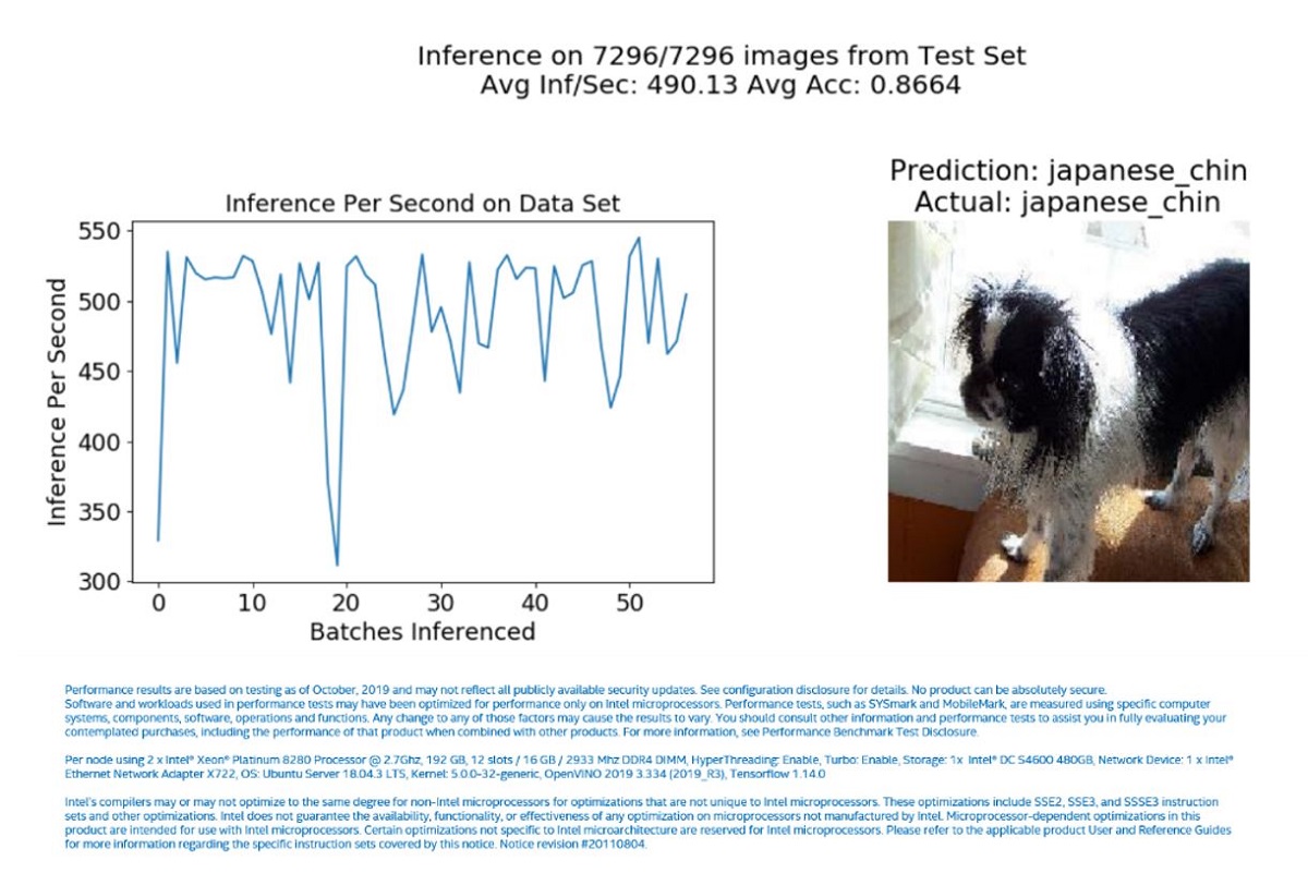
Figure 3. Inference Results with FP32 IR
The plot in Figure 3 shows the measured inference FPS for every batch while running through the entire dataset. In this experiment, the average FPS1 was 490.13, and the overall accuracy of the test set was 0.8664.
The ResNet50 model is used here, and it can be better tuned and trained to increase accuracy. However, in this experiment, we are only interested in the performance of a trained model over a dataset to show how it performs with both FP32 and INT8 IRs.
INT8 Model Inference Stages
This section describes the steps required to run INT8 inference.
- Use the Calibration Tool in the OpenVINO™ toolkit to create the INT8 model.
- Load the quantized IR.
- Run inference with the INT8 IR.
Using the Calibration Tool
The Calibration Tool quantizes a given FP16 or FP32 model and produces a low-precision 8-bit integer (INT8) model while keeping model inputs in the original precision. To learn more about benefits of inference in INT8 precision, refer to Using Low-Precision 8-bit Integer Inference.
You can run the Calibration Tool in two modes: standard and simplified. In standard mode, it performs quantization with a minimal drop in accuracy. In simplified mode, all layers are considered to be executed in INT8 IR, and the tool produces the IR that contains plain statistics for each layer. Because simplified mode can cause a dramatic accuracy drop, use this mode only to understand the potential inference performance gain of your application. To learn more about how to use the Calibration Tool, refer to Calibration Tool.
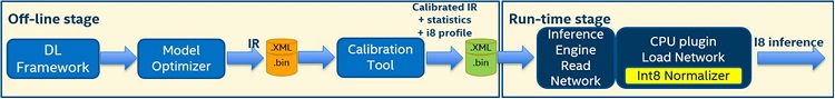
Figure 4. Calibration Tool Flow
Figure 4 summarizes the steps to create the INT8 IR from the same frozen graph. The following steps use the new INT8 IR to perform inference on the same dataset.
Step 1: Convert the Annotations
This step uses the Imagenet style files to create a Pickle file and a Json file; each file contains a subset of the dataset for accuracy checking. We're using a subset of 256 to gather a multiple-of-2 batch size. This will provide some flexibility for annotation file reuse later when creating a model with different batch sizes. Refer to Annotation Converters for further details.
mkdir annotations
python3 /opt/intel/openvino/deployment_tools/tools/accuracy_checker_tool/convert_annotation.py \
    imagenet \
    --annotation_file val.txt \
    --labels_file synset_words.txt \
    --subset 256 \
    --output_dir annotations \
    --annotation_name val.pickle \
    --meta_name val.json
Step 2: Generate the INT8 Model
Using the Calibration Tool to generate the INT8 model requires two files: pets-definition.yml and pets-config.yml. These files contain the information needed to create the IR and they require only a minimum number of parameters when calling the calibrate.py file. Once the calibration is done, the tool will create the .bin or .xml file appended with _i8.
python3 /opt/intel/openvino/deployment_tools/tools/calibration_tool/calibrate.py \
    --config pets-config.yml \
    --definition pets-definition.yml \
    -M /opt/intel/openvino/deployment_tools/model_optimizer/
The following two .yml files serve as an example for your applications:
pets-config.yml
models:
  - name: resnet50

    launchers:
      - framework: dlsdk
        device: CPU
        tf_model: pets.rn50.pb
        adapter: classification
        mo_params:
            data_type: FP32
            input_shape: "(128, 224, 224, 3)"
            mean_values: "(123,117, 104)"
        mo_flags:
          - reverse_input_channels
    datasets:
      - name: pets
pets-definition.yml
launchers:
  - framework: dlsdk
    device: CPU

datasets:
  - name: pets
    data_source: pets_images
    annotation: annotations/val.pickle
    dataset_meta: annotations/val.json
    preprocessing:
      - type: bgr_to_rgb
      - type: normalization
        mean: 123, 117, 104
    metrics:
      - name: accuracy @ top1
        type: accuracy
        top_k: 1
Step 3: Verify the Results
To verify the results using the Accuracy Checker (from the DLDT), run the following command:
 python3 /opt/intel/openvino/deployment_tools/tools/accuracy_checker_tool/accuracy_check.py \
    --config pets-config.yml \
    -d pets-definition.yml \
    -M /opt/intel/openvino/deployment_tools/model_optimizer/
Instantiate the Network and Run Inference
This process uses the same code from above, pulls in the new .bin or .xml files, and uses those files moving forward. Instead of defining arg_model="pets.rn50.xml", the INT8 IRs arg_model="pets.rn50_i8.xml" is loaded and everything else for the inference code will be the same.
Running through the same dataset again, the new application performs as shown in Figure 5. The average FPS[ii] in the run is 1073.38 and the accuracy is 0.8642. Comparing Figures 3 and 5, you can see that there is a clear boost in performance when using INT8 (1073.38/490.13 = 2.19, and the loss in accuracy is 0.8664-0.8642 = 0.0022, which is less than 0.3 percent).

Figure 5. Inference results with INT8 IR
Further Analysis Using OpenVINO Tools
While running our inference application, we found that all the cores were not fully utilized. OpenVINO provides the Benchmark Python* Tool and Benchmark C++ Tool, which perform inference using convolutional neural networks and help you measure the performance of your trained model.
Performance can be measured for two inference modes: synchronous (latency-oriented) and asynchronous (throughput-oriented). The code below demonstrates how to run the FP32 and INT8 IR through the Benchmark Python* Tool and save the outputs into a text file for further analysis.
#Run Benchmark App with FP32 IR
python3 /opt/intel/openvino/deployment_tools/tools/benchmark_tool/benchmark_app.py -m pets.rn50.xml -t 20 2>&1 | tee pets_fp32_benchmark.txt

#Run Benchmark App with INT8 IR
python3 /opt/intel/openvino/deployment_tools/tools/benchmark_tool/benchmark_app.py -m pets.rn50_i8.xml -t 20 2>&1 | tee pets_int8_benchmark.txt
OpenVINO provides a preview release of Deep Learning Workbench, which is another option to run a web-based graphical environment for your models. It helps you measure your model performance on a variety of hardware and can automatically fine-tune the performance of an OpenVINO model by reducing the precision of certain model layers (quantization) from FP32 to INT8. Using this tool, you can experiment with model optimizations and inference options, analyze inference results, and apply an optimal configuration.
Comparison of FP32 Versus INT8 Inference Speed
Figure 6 summarizes the results of the inference FPS metric for all the above experiments. The FP32 and INT8 bars reflect the results from the inference application; they show a boost of approximately 2.19x. The FP32 Streams and INT8 Streams bars show the results from the OpenVINO Benchmark PythonTool and we see a 3.42x boost when comparing FP32 Streams vs INT8 Streams as a result of better CPU core utilization.

Figure 6. FP32 versus INT8 Inference Speeds
Conclusion
This article describes how the use of Intel Distribution of OpenVINO—and the power of vector neural network instructions (VNNI) and Intel® Advanced Vector Extensions 512 (Intel® AVX-512) can accelerate your workload. You can see a clear performance boost with Intel DL-Boost on inference workloads.
Additional Resources
Intel® Distribution of OpenVINO™ Toolkit
Calibration Tool User Guide
Authors
Abdulmecit Gungor is an AI developer evangelist at Intel Corporation. He works closely with the developer community, trains developers, and speaks at universities and conferences on Intel® AI technologies. He has a master’s degree from Purdue University and a bachelor’s degree from City University of Hong Kong. He also holds an academic achievement award from The S. H. Ho Foundation. His interests are end-to-end natural language programming application development on real-life problems, text mining, statistical machine learning, and performance optimization of AI workloads.
Michael Zephyr is an AI developer evangelist in the Architecture, Graphics and Software Group at Intel Corporation. He promotes various Intel® technologies that pertain to machine learning and AI, and he regularly speaks at universities and conferences to help spread AI knowledge. Michael holds a bachelor's degree in computer science from Oregon State University and a master's degree in computer science from the Georgia Institute of Technology. In his free time, you can find him playing board games or video games and lounging with his wife and cat.
Footnotes
1. Performance results are based on testing as of October 2019 and may not reflect all publicly available security updates. See configuration disclosure for details. No product can be absolutely secure.
Software and workloads used in performance tests may have been optimized for performance only on Intel® microprocessors. Performance tests, such as SYSmark* and MobileMark*, are measured using specific computer systems, components, software, operations and functions. Any change to any of those factors may cause the results to vary. You should consult other information and performance tests to assist you in fully evaluating your contemplated purchases, including the performance of that product when combined with other products. For more information, see Performance Benchmark Test Disclosure.
Per node using 2 x Intel® Xeon® Platinum 8280 Processor @ 2.7Ghz, 192 GB, 12 slots / 16 GB / 2933 Mhz DDR4 DIMM, HyperThreading: Enable, Turbo: Enable, Storage: 1x Intel® DC S4600 480GB, Network Device: 1 x Intel® Ethernet Network Adapter X722, OS: Ubuntu Server 18.04.3 LTS, Kernel: 5.0.0-32-generic, OpenVINO 2019 3.334 (2019_R3), and Tensorflow 1.14.