A key design goal of Simics® software is that it should be a fast virtual platform. Keeping Simics fast and making it faster is a constant concern and point of pride for the Simics development team.

Thus, it was with some concern that I heard a user praise Simics at an office party, saying, “Simics was fantastic. It solved my problem. It just took a few weeks to run.” Weeks? A Simics run that takes minutes is completely normal. Hours are common too. Days are starting to stretch it. But weeks? Something wasn’t right. Not for a fast functional run with no added details or heavy logging or instrumentation.
What was going on to make Simics run for such a long time? The analysis of this performance problem turned into a month-long odyssey. It offers an object lesson in the value of the classic debug advice to “Quit thinking and look.” Don’t form conclusions prematurely. Look at what is going on instead of guessing and cooking up theoretical scenarios. Sound advice that I have been telling people for a long time, and that I immediately proceeded not to follow.
“It Must be Temporal Decoupling”
In this case, I was convinced from the start that the problem was temporal decoupling. The program that took weeks to run on Simics was a multithreaded producer-consumer setup, with one thread feeding data for another thread to process.
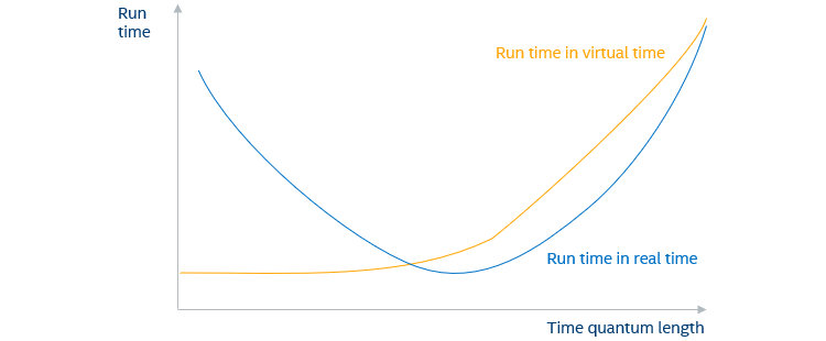
Figure 1: Typical behavior for a program that is affected by temporal decoupling.
This kind of software pattern has been known in the past to exhibit longer run times when the time quantum length increases, resulting the familiar plot sketched in Figure 1: the virtual run time of a software load increases with the length of a time quantum, but the simulation run time first decreases as temporal decoupling increases performance, and the virtual run time only increases slowly. However, beyond a certain point, the simulation run time increases when the cost of simulating additional virtual time starts to dominate.
Given this past experience on supposedly similar software, the obvious question became where to find the optimal point for this workload? The plan was to perform a set of runs with different time quantum lengths to get to the curves in Figure 1 and find the minimal real-world run time.
The next step was to look at the actual situation.
Running built-in Simics performance analysis tools provided an initial insight into why the simulation was slow on the workload. It turned out that Simics VMP was not being used as much as expected. This was because the target system being modeled used new Intel Architecture instructions not found on the host. This significant slow-down had nothing at all to do with temporal decoupling; it was just a matter of selecting a good host to run Simics (which is seen very often).
Thus, the first performance optimization was to make sure that the host system running Simics was of the same generation as the target system being simulated. With this change, the workload ran several times faster. It still seemed to take way too long to run, however.
Next, an automatic performance test script was created to run the simulation with various time quantum lengths. It scripted all inputs, detected the end of the target software run, and logged the run time in both virtual and host time. A large set of runs were made, varying the time quantum from very short to very long—we expected to see a graph like Figure 1.
It was an epic simulation campaign. While the shortest runs only required seven hours to finish, the longest run was cancelled after 21 days and only getting two thirds to the finish line. So, what did I see?
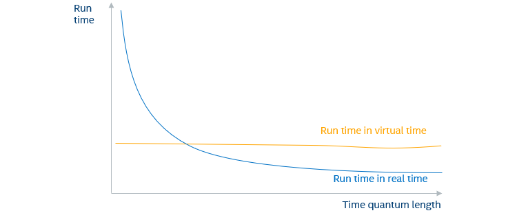
Figure 2: Observed behavior when varying the time quantum length
Figure 2 shows a sketch of the measured run times: the virtual run time was essentially constant across time quantum lengths—surprisingly stable. Increasing the time quantum made the run finish faster, just like it is supposed to do (because longer time quanta usually give higher simulation performance).
After three weeks of measuring Simics performance for this workload, the result was a big question mark. So much for self-confident proclamations of the self-evident cause for the performance problem.
“Quit Thinking and Look”
Looking at the data again provided a new angle. The actual time it took to run the workload on the Simics target was quite a bit larger than what it took to run on a real host. Typically, when a workload is run on Simics and takes, say, 10 minutes to complete on a real host, the expectation is that it will take something similar on Simics. Not precisely the same, because Simics is not a timing-accurate simulator, but at least reasonably close.
In this case, the workload run time was way off—between 10x and 100x more than the run time in the real world. My initial guess was that the virtual execution time would be off, but that it would get back to close to what was seen in the real world by reducing the time quantum. But Figure 2 effectively disproved that. Note that this should have been considered after doing only a few runs, no need to wait for the three weeks long slow run.
What was going on?
A New Angle and More Measurements
Simics attempts to optimize the performance of common polling loops in software that uses the read time-stamp counter (RDTSC) instruction by adding a delay to each read. In such loops, software reads the RDTSC waiting for a certain value to appear. By making each execution of RDTSC take a rather long virtual time (the default is 20,000 cycles), software gets to the end of a polling loop in fewer iterations while still getting approximately the right timing. It works well for most software and provides a useful performance improvement.
However, this particular workload seems to use RDTSC in a very different way. As sketched in Figure 3, lowering the RDTSC delay reduced the virtual run time, and it also reduced the real-world execution time of the workload.
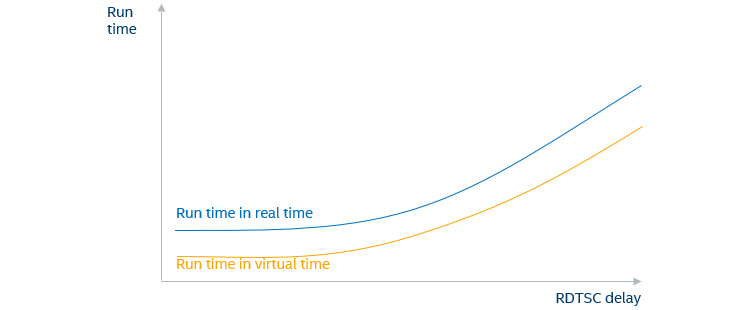
Figure 3: Observed behavior when varying RDTSC delay (time quantum constant)
Thus, the answer seemed clear: for this workload, the best performance optimization was to dial down the Simics RDTSC delay (which is under user control and can be changed at any point during a run). This got the virtual run time down to about the same as the workload observed on real hardware, and the simulation run time down to a reasonable few hours. All around a better result: a run that more closely matches hardware, and runs in hours instead of weeks.
Mission accomplished and time to go home? Not quite.
“Temporal Decoupling Must Still Have Some Effect”
There was still a nagging sense in my mind that temporal decoupling should interact with this somehow. It just couldn’t not be so. Right?
So, I did another round of simulation runs with different time quantum values for the same RDTSC delay (across multiple RDTSC delays, just to be sure). This took another few days of experiments, but in the end, there was nothing to show for it. Varying the time quantum had no effect whatsoever on the virtual run time of the workload. Zero. So much for my pet hypothesis.
Giving Up and Concluding
I learned something from this investigation. I hope that this story serves as a cautionary tale about the importance of keeping an open mind when investigating software issues, be they functional bugs or performance problems: don’t think before you have data to work from, and go where the data leads. It is easy to waste a lot of time trying to prove an incorrect hypothesis, and past experience is not always a reliable guide to a current problem.
You cannot fix software with eloquent rhetoric and elegant theories. It does not care what you say.
Performance tuning knobs are present in tools like Simics for a reason. Different workloads might react in different ways to different settings, and the defaults, while generally good, are sometimes not optimal for a particular case. That is an eternal issue confounding software performance: workloads are not all created equal, and “the best” settings and optimizations are likely to vary.
Thus, the advice is always: Quit thinking, and look at what is going on, and work from that.
Related Content
Simics 6, A Deeper Look at how Software Uses Hardware: The new Simics 6 makes it easy for developers to investigate and quantify how software uses the programming registers of hardware devices.
Using Clear Linux* for Teaching Virtual Platforms: Moving to Clear Linux was really all about how to configure and use a modern Linux.
Containerizing Wind River Simics® Virtual Platforms (Part 1): Developers can gain major benefits from using containers with Wind River* Simics* virtual platforms.
Using Wind River* Simics* with Containers (Part 2): Wind River Simics has advantages over using hardware for debugging, fault injection, pre-silicon software readiness, and more.
Author
 Dr. Jakob Engblom is a product management engineer for the Simics virtual platform tool, and an Intel® Software Evangelist. He got his first computer in 1983 and has been programming ever since. Professionally, his main focus has been simulation and programming tools for the past two decades. He looks at how simulation in all forms can be used to improve software and system development, from the smallest IoT nodes to the biggest servers, across the hardware-software stack from firmware up to application programs, and across the product life cycle from architecture and pre-silicon to the maintenance of shipping legacy systems. His professional interests include simulation technology, debugging, multicore and parallel systems, cybersecurity, domain-specific modeling, programming tools, computer architecture, and software testing. Jakob has more than 100 published articles and papers and is a regular speaker at industry and academic conferences. He holds a PhD in Computer Systems from Uppsala University, Sweden.