For applications such as high frequency trading (HFT), search engines and telecommunications, it is essential that latency can be minimized. My previous article Optimizing Computer Applications for Latency, looked at the architecture choices that support a low latency application. This article builds on that to show how latency can be measured and tuned within the application software.
Using Intel® VTune™ Amplifier
Intel VTune Amplifier can collect and display a lot of useful data about an application’s performance. You can run a number of pre-defined collections (such as parallelism and memory analysis) and see thread synchronization on a timeline. You can break down activity by process, thread, module, function, or core, and break it down by bottleneck too (memory bandwidth, cache misses, and front-end stalls).
Intel VTune Amplifier can be used to identify many important performance issues, but it struggles with analyzing intervals measured in microseconds. Intel VTune Amplifier uses periodic interrupts to collect data and save it. The frequency of those interrupts is limited to roughly one collection point per 100 microseconds per core. While you can filter the data to observe some of the outliers, the data on any single outlier will be limited, and some might be missed by the sampling frequency.
You can download a free trial of Intel VTune Amplifier. Read about the VTune Amplifier capabilities.
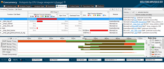
Figure 1. Intel VTune Amplifier XE 2017, showing hotspots (above) and concurrency (below) analyses
Using Intel® Processor Trace Technology
The introduction of Intel® Processor Trace (Intel® PT) technology in the Broadwell architecture, for example in the Intel® Xeon® processor E5-2600 v4, makes it possible to analyze outliers in low latency applications. Intel® PT is a hardware feature that logs information about software execution with minimal impact on system execution. It supports control flow tracing, so decoder software can be used to determine the exact flow of the software execution, including branches taken and not taken, based on the trace log. Intel PT can store both cycle count and timestamp information for deep performance analysis. If you can time stamp other measurements, traces, and screenshots you can synchronize the Intel PT data with them. The granularity of a capture is a basic block. Intel PT is supported by the “perf” performance analysis tool in Linux*.
Typical Low Latency Application Issues
Low latency applications can suffer from the same bottlenecks as any kind of application, including:
- Using excessive system library calls (such as inefficient memory allocations or string operations)
- Using outdated instruction sets, because of obsolete compilers or compiler options
- Memory and other runtime issues leading to execution stalls
On top of those, latency-sensitive applications have their own specific issues. Unlike in high-performance computing (HPC) applications, where loop bodies are usually small, the loop body in a low latency application usually covers a packet processing instruction path. In most cases, this leads to heavy front-end stalls because the decoded instructions for the entire packet processing path do not fit into the instruction (uop) cache. That means instructions have to be decoded on the fly for each loop iteration. Between 40 and 50 per cent of CPU cycles can stall due to the lack of instructions to execute.
Another specific problem is due to inefficient thread synchronization. The impact of this usually increases with a higher packet/transaction rate. Higher latency may lead to a limited throughput as well, making the application less able to handle bursts of activity. One example I’ve seen in customer code is guarding a single-threaded queue with a lock to use it in a multithreaded environment. That’s hugely inefficient. Using a good multithreaded queue, we’ve been able to improve throughput from 4,000 to 130,000 messages per second. Another common issue is using thread synchronization primitives that go to kernel sleep mode immediately or too soon. Every wake-up from kernel sleep takes at least 1.2 microseconds.
One of the goals of a low latency application is to reduce the quantity and extent of outliers. Typical reasons for jitter (in descending order) are:
- Thread oversubscriptions, accounting for a few milliseconds
- Runtime garbage collector activities, accounting for a few milliseconds
- Kernel activities, accounting for up to 100s of microseconds
- Power-saving states:
- CPU C-states, accounting for 10s to 100s of microseconds
- Memory states
- PCI-e states
-
Turbo mode frequency switches, accounting for 7 microseconds
-
Interrupts, IO, timers: responsible for up to a few microseconds
Tuning the Application
Application tuning should begin by tackling any issues found by Intel VTune. Start with the top hotspots and, where possible, eliminate or reduce excessive activities and CPU stalls. This has been widely covered by others before, so I won’t repeat their work here. If you’re new to Intel VTune, there’s a Getting Started guide.
In this article, we will focus on the specifics for low latency applications. The biggest issue arises from front-end stalls in the instruction decoding pipeline. This issue is difficult to address, and results from the loop body being too big for the uop cache. One approach that might help is to split the packet processing loop and process it by a number of threads passing execution from one another. There will be a synchronization overhead, but if the instruction sequence fits into a few uop caches (each thread bound to different cores, one cache per thread), it may well be worth the exercise.
Thread synchronization issues are somewhat difficult to monitor. Intel VTune Amplifier has a collection that captures all standard thread sync events (Windows* Thread API, pthreads* API, Intel® Threading Building Blocks and OpenMP*). It helps to understand what is going on in the application, but deeper analysis is required to see if a thread sync model introduces any limitations. This is non-trivial exercise requiring quite some expertise. The best advice is to use a highly performant threading solution.
An interesting topic is thread affinities. For complex systems with multiple thread synchronization patterns along the workflow, setting the best affinities may bring some benefit. A synchronization object is a variable or data structure, plus its associated lock/release functionality. Threads synchronized on a particular object should be pinned to a core of the same socket, but they don’t need to be on the same core. Generally the goal of this exercise is to keep thread synchronization on a particular object local to one of the sockets, because cross-socket thread sync is much costlier.
Tackling Outliers in Virtual Machines
If the application runs in a Java* or .NET* virtual machine, the virtual machine needs to be tuned. The garbage collector settings are particularly important. For example, try tuning the tenuring threshold to avoid unnecessary moves of long-lived objects. This often helps to reduce latency and cut outliers down.
One useful technology introduced in the Intel® Xeon® processor E5-2600 v4 product family is Cache Allocation Technology. It allows a certain amount of last level cache (LLC) to be dedicated to a particular core, process, or thread, or to a group of them. For example, a low latency application might get exclusive use of part of the cache so anything else running on the system won’t be able to evict its data.
Another interesting technique is to lock the hottest data in the LLC “indefinitely”. This is a particularly useful technique for outlier reduction. The hottest data is usually considered to be the data that’s accessed most often, but for low latency applications it can instead be the data that is on a critical latency path. A cache miss costs roughly 50 to 100 nanoseconds, so a few cache misses can cause an outlier. By ensuring that critical data is locked in the cache, we can reduce the number and intensity of outliers.
For more information on Cache Allocation Technology, see Using Hardware Features in Intel® Architecture to Achieve High Performance in NFV.
Exercise
Let’s play with a code sample implementing a lockless single-producer single-consumer queue. Download![]() Download
Download
To start, grab the source code for the test case from the download link above. Build it like this:
gcc spsc.c -lpthread –lm -o spsc
Or
icc spsc.c -lpthread –lm -o spsc
Here’s how you run the spsc test case:
./spsc 100000 10 100000
The parameters are: numofPacketsToSend bufferSize numofPacketsPerSecond. You can experiment with different numbers.
Let’s check how the latency is affected by CPU power-saving settings. Set everything in the BIOS to maximum performance, as described in Part 1 of this series. Specifically, CPU C-states must be set to off and the correct power mode should be used, as described in the Kernel Tuning section. Also, ensure that cpuspeed is off.
Next, set the CPU scaling governor to powersave. In this code, the index i goes up to the number of cores:
for ((i=0; i<23; i++)); do echo powersave > /sys/devices/system/cpu/cpu$i/cpufreq/scaling_governor; done
Then set all threads to stay on the same NUMA node using taskset, and run the test case:
taskset –c 0,1 ./spsc 1000000 10 1000000
On a server based on the Intel® Xeon® Processor E5-2697 v2, running at 2.70GHz, we see the following results for average latency with and without outliers, the highest and lowest latency, the number of outliers and the standard deviation (with and without outliers). All measurements are in microseconds:
taskset -c 0,1 ./spsc 1000000 10 1000000
Avg lat = 0.274690, Avg lat w/o outliers = 0.234502, lowest lat = 0.133645, highest lat = 852.247954, outliers = 4023
Stdev = 0.001214, stdev w/o outliers = 0.001015
Now set the performance mode (overwriting the powersave mode) and run the test again:
for ((i=0; i<23; i++)); do echo performance > /sys/devices/system/cpu/cpu$i/cpufreq/scaling_governor; done
taskset -c 0,1 ./spsc 1000000 10 1000000
Avg lat = 0.067001, Avg lat w/o outliers = 0.051926, lowest lat = 0.045660, highest lat = 422.293023, outliers = 1461
Stdev = 0.000455, stdev w/o outliers = 0.000560
As you can see all the performance metrics improved significantly when we enabled performance mode: the average, the lowest and highest latency, and the number of outliers. (Table 1 summarizes all the results from this exercise for easy comparison).
Let’s compare how the latency is affected by a NUMA locality. I’m assuming you have a machine with more than one processor. We’ve already run the test case bound to a single NUMA node.
Let’s run the test case over two nodes:
taskset -c 8,16 ./spsc 1000000 10 1000000
Avg lat = 0.248679, Avg lat w/o outliers = 0.233011, lowest lat = 0.069047, highest lat = 415.176207, outliers = 1926
Stdev = 0.000901, stdev w/o outliers = 0.001103
All of the metrics, except for the highest latency, are better on a single NUMA node. This results from the cost of communicating with another node, because data needs to be transferred over Intel® QuickPath Interconnect (Intel® QPI) link and over all parts of the cache coherency mechanism.
Don’t be surprised that the highest latency is lower on two nodes. You can run the test multiple times and verify that the highest latency outliers are roughly the same for both one node and two nodes. The lower value shown here for two nodes is most likely a coincidence. The outliers are two to three orders of magnitude higher than the average latency, which shows that NUMA locality doesn’t matter for the highest latency. The outliers are caused by kernel activities that are not related to NUMA.
| Test | Avg Lat | Avg Lat w/o Outliers | lowest Lat | highest Lat | outliers | Stdev | Stdev w/o Outliers |
| Powersave | 0.274690 | 0.234502 | 0.133645 | 852.247954 | 4023 | 0.001214 | 0.001015 |
| Performance 1 node | 0.067001 | 0.051926 | 0.045660 | 422.293023 | 1461 | 0.000455 | 0.000560 |
| Performance 2 nodes | 0.248679 | 0.233011 | 0.069047 | 415.176207 | 1926 | 0.000901 | 0.001103 |
Table 1: The results of the latency tests conducted under different conditions, measured in microseconds.
I also recommend playing with Linux perf to monitor outliers. Intel PT support starts with Kernel 4.1. You need to add timestamps (start, stop) for all latency intervals, identify a particular outlier and then drill down into perf data to see what was going on during the interval of the outlier.
For more information, see https://github.com/torvalds/linux/blob/master/tools/perf/Documentation/intel-pt.txt.
Conclusion
This two-part article has summarized some of the approaches you can take, and tools you can use, when tuning applications and hardware for low latency. Using the worked example here, you can quickly see the impact of NUMA locality and powersave mode, and you can use the test case to experiment with other settings, and quickly see the impact they can have on latency.
"