Overview
Data discretization is a common pre-processing step in machine learning or data mining process flows. The greatest challenge in discretizing (binning) a dataset is preserving the original data distribution, while maintaining a reasonable bin size. Intel® Optimized Data Discretization Reference Implementation does the following:
- Automatically discretizes or develops a histogram of data for advanced processing and analysis.
- Introduces an API interface to return optimal bin size for a given set of data.
- Provides a Python* GUI app demonstrating API usage along with visual histogram comparison with state-of-the-art available method.
- Gives a reference microservice implementation to showcase API usage in client/server scenario.
- Supports multiple data publishers such as Microsoft* Excel*, CSV and InfluxDB*.
Select Configure & Download to download the reference implementation and the Intel® Optimized Data Discretization Software for evaluation and testing of your Intel®-based solution.
- Time to Complete: Approximately 15-30 minutes
- Programming Language: Python* 3.8
- Available Software: Ubuntu* 20.04
Target System Requirements
- Ubuntu* 20.04
- 6th to 11th Generation Intel® Core™ processors
- This reference implementation will work on any Intel®-based solution. See the Recommended Hardware page for suggestions.
How It Works
Two types of reference clients are included in this reference implementation:
- Standalone Application: Demonstrates API invocation via Python GUI application.
- Microservice: Showcases client server scenario usage with knowledge discovery API calling at the backend by server code.
Standalone Application
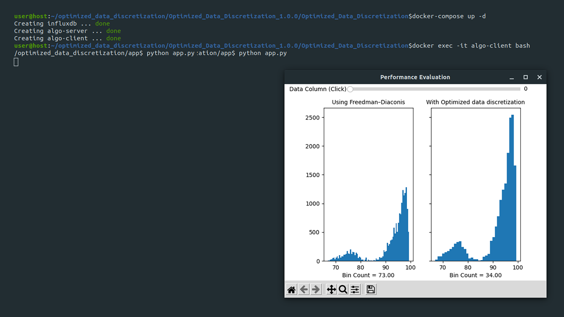
Standalone Application is released as a Python script. It displays two side-by-side histograms for comparison across series of datapoints selected via on screen slider.
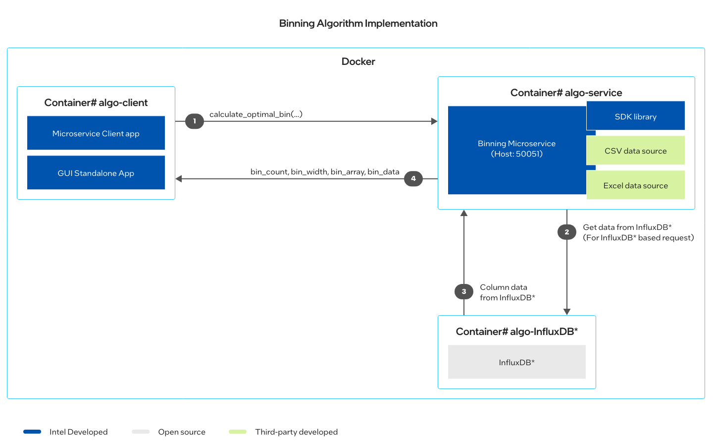
Microservice
Three containers are created as result of the docker-compose up command:
- Server container with microservice instance.
- InfluxDB container to support Influxdb data publisher.
- Client container to issue requests.
The Server and Client containers are created using the same Docker* image. The microservice server instance runs as part of docker-compose up command in algo-server container.
A microservice-based solution demonstrates an end-to-end pipeline utilizing discretization API to calculate optimal bin for a given set of data. The service offers data inputs from either CSV, Excel, or InfluxDB. Client, Server and InfluxDB are running in their respective Docker containers.
Three containers are created out of two images:
- algo:latest image provides the foundation for client and server containers.
- influxdb:1.1.1 image is used to create the influxdb container.
Histogram
The reference implementation automatically discretizes or develops a histogram of data for advanced processing and analysis.
A histogram is a graphical representation of the distribution of numerical data. It is an estimate of the probability distribution of a continuous variable. Histograms are an effective tool to categorize or discretize real data. Categorizing real data into discrete bins is required for multiple machine learning and data mining methods. Binning real data into a fewer number of categories allows for better clustering and pattern matching by summarizing the raw data into meaningful segments, specifically when the data range is very large and the number of data samples is very high.
However, the greatest challenge in creating a histogram is the determination of the bin widths. The bin width should not be so small that the histogram loses its purpose, and on the other hand, should not be so large that the histogram deviates from the inherent distribution of the raw data. The histogram should be able to represent the raw data distribution, while simultaneously proving meaningful binning of the data into fewer categories for efficient data correlation and association, which is required for many types of machine learning and data mining methods. Hence, the problem reduces to identifying the optimal bin width.
Research focused on selecting an optimal bin width is ongoing. However, most of the published research looks at determining the bin width based on minimizing the difference in distribution between the original data and the histogram. As a result, the bin widths determined by these methods are often very small and not useful when the data range is very large.
Developing a meaningful histogram is key to the success of the subsequent data processing methods. This RI addresses this issue and provides a method that preserves the inherent resolution in the data or data distribution and simultaneously ensures a reasonably large bin width, thus allowing a meaningful summarization of the data. This method is an optimization between two competing factors: the best representation of data distribution and the bin width size.
The proposed method has been successfully tested with a wide range of data and compared with the methods published in literature.
Comparative Results
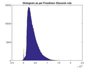
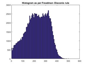
Figures 2, 4, and 6 below present the histograms obtained by a well-known method in literature (Freedman-Diaconis rule).
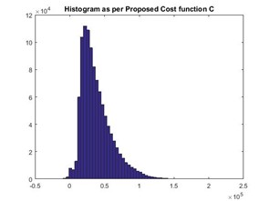
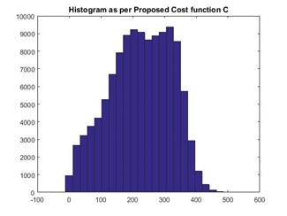
Figures 3, 5, and 7 below show the histograms obtained by the reference implementation for the same data set.
The bin sizes obtained under each case are provided below. We observed that the bin sizes obtained by the RI are significantly larger than that obtained by the Freedman-Diaconis rule, while still preserving the data distribution.
Test Case 1
In this test case, the Freedman-Diaconis rule obtained bin width: 533.77, while the RI obtained bin width: 4202.60.
|
|
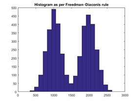
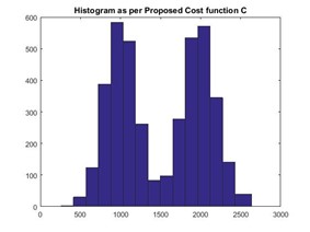
Test Case 2
In this test case, the Freedman-Diaconis rule obtained bin width: 6.08, while the RI obtained bin width: 22.59.
|
|
Test Case 3
In this test case, the Freedman-Diaconis rule obtained bin width: 126, while the RI obtained bin width: 152.10.
|
|
Get Started
Install the Reference Implementation
Select Configure & Download to download the reference implementation and the Intel® Optimized Data Discretization Software for evaluation and testing of your Intel®-based solution.
- Open a new terminal, go to the downloaded folder and unzip the RI package.
unzip optimized_data_discretization.zip - Go to the optimized_data_discretization directory.
cd optimized_data_discretization - Change permission of the executable edgesoftware file.
chmod 755 edgesoftware - Run the command below to install the reference implementation:
./edgesoftware install - During the installation, you will be prompted for the Product Key. The Product Key is contained in the email you received from Intel confirming your download.
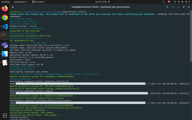
Figure 8: Product Key
- When the installation is complete, you see the message Installation of package complete and the installation status for each module.
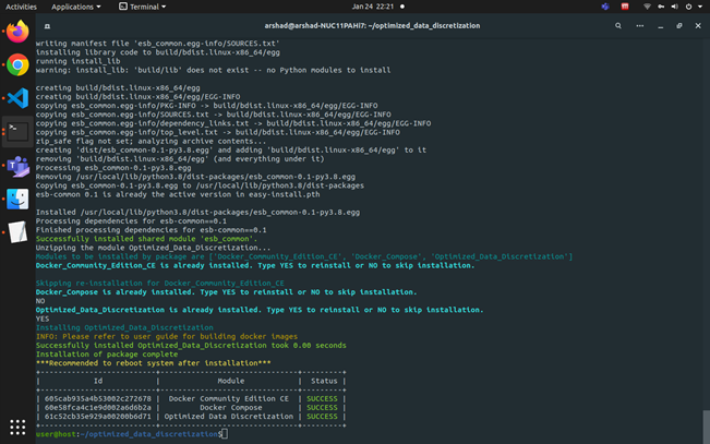
Figure 9: Installation Complete
Run the Application
- Go to the working directory:
cd optimized_data_discretization/Optimized_Data_Discretization_1.0.0/Optimized_Data_Discretization - Build Docker images with the following command:
chmod 777 buildimages.sh ./buildimages.sh - Set environment variable DOCKER_USER to current host user. This will enable docker-compose to run containers under current host user context. This export command can be added to bash login script for persistence, otherwise you will need to run it for each new session.
export DOCKER_USER=”$(id -u):$(id -g)” - Run the command below to initialize containers:
docker-compose up -d - Attach to the container using the following command:
docker exec -it algo-client bash
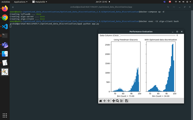
Standalone Application
In the below example, the state-of-the-art Freedman-Diaconis algorithm returned 73 bins and the Intel® Optimized Data Discretization RI calculated 34 bins while preserving the data distribution.
cd /optimized_data_discretization/app
python app.py
Microservice
Attach to client container and run client.py from it.
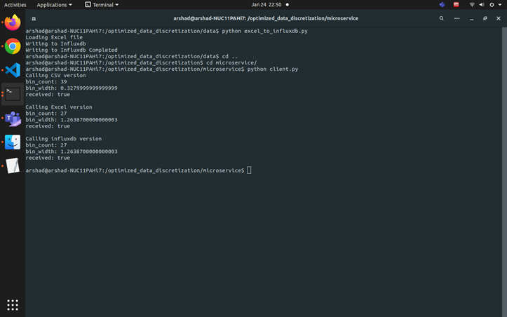
Fill up the influxdb database with values. You need to do this step every time you initiate a Docker session and the values are available until you end the Docker session.
cd /optimized_data_discretization/data
python excel_to_influxdb.py
Run microservice client with the commands:
cd /optimized_data_discretization/microservice
python client.py
Invoking client.py will send a request to the server for histogram bin calculation on Excel data publisher.
API Usage
The API library is provided as an .so file. The docker-compose.yml file sets up PYTHONPATH to lib directory for standalone application and microservice server containers for API invocation.
Regular usage of the API will require you to set up an environment variable as shown below:
export PYTHONPATH=<.so location>
The function below takes in an array vector of data and based on an innovative Cost function returns the optimal number of categories, width of each category, boundary values of each bin and the data belonging to each bin.
Function Prototype
[bin_count, bin_width, bin_array, bin_data] automated_optimal_binning(datapoints)
Parameters:
datapoints: data points as numpy list
Return values:
bin_count: Optimal bin count value
bin_width: Bin widths
bin_array: edge values
bin_data: Histogram data
Summary and Next Steps
With this reference implementation you successfully evaluated different data distributions that have a wide range of values. Besides approximating the distribution, the reference implementation also optimizes the bin width. This method is best suited for cases where grouping of data into an optimal number of bins is essential for the success of subsequent data processes. One such application is associative memory techniques, which keeps a record of co-occurrences of values or entities for building associations. Also methods which are based on similarities in values, entities for developing recommendation engines, or for clustering profiles or mining patterns.
Learn More
To continue learning, see the following guides and software resources:
- Freedman-Diaconis rule on Wikipedia
Support Forum
If you're unable to resolve your issues, contact the Support Forum.