Introduction
Imperator: Rome is the newest grand strategy game from Paradox* Development Studio, and we have been working together on its performance on Intel® Iris™ Pro Graphics 580. It was an interesting journey because we had to take a slightly different route in terms of the performance analysis. The issue we encountered wasn’t necessarily bad performance, but rather an occasional stuttering caused by the Gradient Borders rendering system, which made us redefine what performance really is. Thanks to the collaboration between Intel and Paradox developers you can now enjoy the game with a smooth framerate on a wide variety of Intel’s integrated graphics hardware.
The article you are about to read is a reflection on this collaboration. First, we’ll use classic performance analysis and see what conclusions we can get from there. Then, we’ll follow up with how we discovered the cause of the stuttering and we’ll question a classic definition of performance. Then, with a little technical background beforehand, we’ll look at the problematic system in detail, we’ll learn what it does and how it works. Finally, we’ll discuss the optimizations that were introduced and the results we were able to achieve.
Initial Performance Evaluation
One of the first things that we developer relations engineers try to determine when we start working on a game is what limits the performance. We use the term GPU-bound or CPU-bound which, loosely translated, means that the highest negative impact on performance is either on the GPU or the CPU. Those two pieces of hardware are usually the main suspects when we look for performance issues.
The general rule of determining the limiting factor is rather simple – if the GPU is busy for at least 95% of the time, then the game is GPU-bound, if not – then we are probably CPU-bound. But what if this is not all there is when it comes to the performance? What if “good performance” is more than the average number of frames per second?
There are many tools to help establish performance-limiting factors, but I personally prefer GPUView. It’s a free profiler that comes with Windows* Assessment and Deployment Kit (Windows ADK). It can give you a quick overview of what is happening on both the CPU and GPU which makes it perfect for game performance analysis. It can also show how much work both GPU and CPU threads need to process.
I collected the GPUView trace of Imperator: Rome (Pompey patch) - the game was in Pause mode which stops all the ongoing CPU simulations and I was panning the camera over Egypt, one of the special areas in the game with dedicated assets.
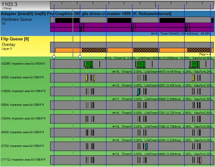
Figure 1. GPUView trace of the game in Pause mode. It represents three rendered frames, shows the work on the GPU as well as active threads.
Figure 1 exhibits the trace with three frames that were presented on the screen – as you can tell by looking at the Flip Queue. Flip Queues show the relationship between Vertical Sync (VSync) and the data that the application presents on the screen. For better presentation, you can toggle VSync events—they are represented by vertical blue lines. You can also see that the Flip Queue bars are divided into two sections. A solid color section represents the time spent on producing the content for the display, usually done by the Desktop Windows Manager (DWM), and the crosshatched section is the idle time where this data waits for the VSync event.
For this specific period, the GPU is 99.66% busy. You can see that value in the lower right corner of the Hardware Queue section. By the definition mentioned earlier this makes the game GPU-bound. That means that game workload execution depends entirely on the GPU efficiency and in turn also means that optimizing GPU content will improve the performance while optimizing CPU workload won’t.
Next, let’s look at the green sections which represent running CPU threads. The thread with the most work is almost 15% busy, while worker threads are around 3% busy. This completes the assessment – we are sure that the game is GPU-bound, and the CPU work is not even close to impact the performance.
Next, let’s take a look at the same thing, but this time with a CPU simulation going on in the background (figure 2). Playing as Rome, during the early game, I’ve started a war with the Samnites as soon as I got casus belli on them, and my subjects joined me. There is a battle going on between my main Roman army of 18,000 men and their army of 8,000 men, as well as a siege of a fortress. At this point the game is in Play mode.
The GPU was busy 99% of the time, which would indicate the game is still GPU-bound, even with the running simulation. The thread with the biggest workload in this timeframe is now 32% busy (in Pause mode it was only 15%). It looks like running the simulation had a significant impact on the CPU. However, the game is still GPU-bound.
Now we know everything, it’s time for the initial performance evaluation. On Intel Iris Pro Graphics 580, Imperator: Rome (Pompey patch) was clearly GPU-bound, no matter whether we were in Pause or Play mode. The GPU was the main bottleneck and theoretically was the best place to target for performance optimizations.
But what was the actual performance? Well, it was very good—the average score achieved in testing was around 30 Frames Per Second (FPS) which means that the game was performing well. What was the problem then? Doesn’t 30 FPS mean that the performance is good, and the game is playable?
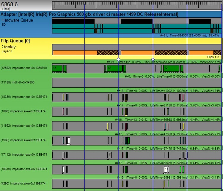
Figure 2. GPUView trace of the game in Play mode. Captured early in the game, during a war between Romans and Samnites, with an ongoing land battle and siege.
Performance Stuttering Discovery
Even though the report said the performance was good, something wasn’t right. In Pause mode I was able to play without any performance issues. When I hit the Play button it was still fine, but as soon as I started to pan the camera around, every couple of frames there was a performance hiccup—it felt like the game was skipping a frame or two. And when I paused the game yet again, the issue disappeared. To better visualize the problem, I’ve collected some data using PresentMon*, a free tool that helps with performance measurements. The chart on Figure 3 shows the time in milliseconds that has passed between presents on the Y-axis, and the frame number on the X-axis.
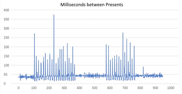
Figure 3. Graph representing milliseconds between presents. Notice the distinct sections with big performance variations, which start when entering Play mode and stop when entering Pause mode.
Looking at this picture I started to wonder – maybe the world of performance is not as black and white as I initially thought. On average we had 30 FPS, but nevertheless the performance didn’t “feel” right, and I wasn’t able to fully immerse myself and enjoy the game. Additionally, the initial performance evaluation showed that we were completely GPU-bound and suddenly it looked like CPU simulation was spoiling it, at least periodically.
At first, I thought that since the problem appeared along with the CPU simulation, it must be related to the CPU workload. Perhaps some very intensive computation was kicking in which potentially was making the game periodically CPU-bound, or maybe there was some kind of CPU work that needed to be in sync with the GPU and was therefore blocking its execution. To investigate that I collected a trace with Intel® VTune™ Profiler, a free CPU profiler tool.
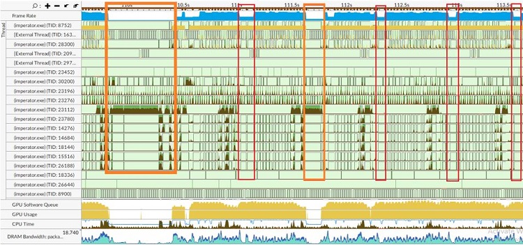
Figure 4. An Intel® VTune™ Profiler trace captured on entering Play mode in the game. Orange and red boxes represent moments where the framerate was dropping.
It turned out that none of the options I'd considered were the issue. Figure 4 presents the Frame Rate in the first row with a blue graph. I’ve marked the slower periods with orange and red boxes. In the orange boxes you can see that the dip in performance is strictly correlated with extensive CPU activity, but in the red boxes it is not. Moreover, there were only two times where the orange boxes appeared—at the beginning, just after entering Play mode. The rest of the trace contained elements that were the same as those in the red boxes.
I presented these results to the Paradox developers. It turns out that the orange boxes represent the situation when simulation initialization takes place. The busiest thread is most likely a so-called Session Thread, responsible for executing gameplay commands. The orange boxes represent the first unpausing in the new game and the Session Thread was doing some initial setup during the first update which caused framerate drop. The session thread will halt the Render and Main Thread which are responsible for the Graphics User Interface (GUI) because the game state is locked when it is updated and when it is locked the GUI can’t query information, so it really shouldn’t present anything.
Interesting—the short-term CPU-bound performance wasn’t causing this permanent hiccup. If it were, then in the red boxes we should have seen a big chunk of continuous work on a single thread while the GPU was stalled. There was only one more thing left to test – the GPU. Using internal tools, I’ve recorded a piece of gameplay in a form of a list of DirectX* API calls. This is a technique we use to analyze GPU-bound workloads. The technique simply records API calls with all the relevant data, meaning this measure the workload as if you had an infinitely fast CPU that didn’t impact performance at all. I replayed the stream, collected the data and analyzed the results.
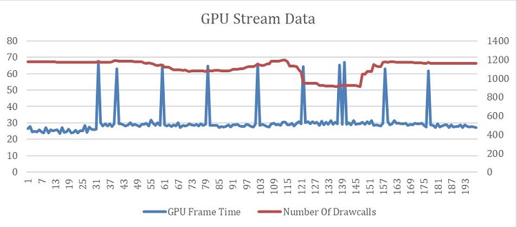
Figure 5. Frame time and number of drawcalls from a GPU stream.
It looks like I’ve found the culprit. Every few frames, the GPU had around twice as much work to do. This can happen sometimes when there are some additional drawcalls to process for example from non-culled objects. I checked that theory and I noticed that the number of drawcalls wasn’t related to performance peaks.
I was getting closer to the root cause. There was some additional work on the GPU every couple of frames and it wasn’t many additional draw calls. There might be just a couple of additional drawcalls in those frames or some of the drawcalls were much longer than usual. Using Intel® Graphics Performance Analyzers (Intel® GPA), I was able to capture one of those frames from the stream (figure 6).
Finally, I found the cause of the stuttering. There were in fact seven additional drawcalls in that frame. Their execution took almost 40 ms which would explain this “missing frame” feeling I had at the beginning. Rendering this one frame took the same amount of time as rendering two regular frames. I reported my findings back to Paradox, and we finally knew what was happening—the Border Rendering System was taking excessively long on the GPU. I asked one of the Paradox developers, Daniel Eriksson, to explain this system a little bit more.
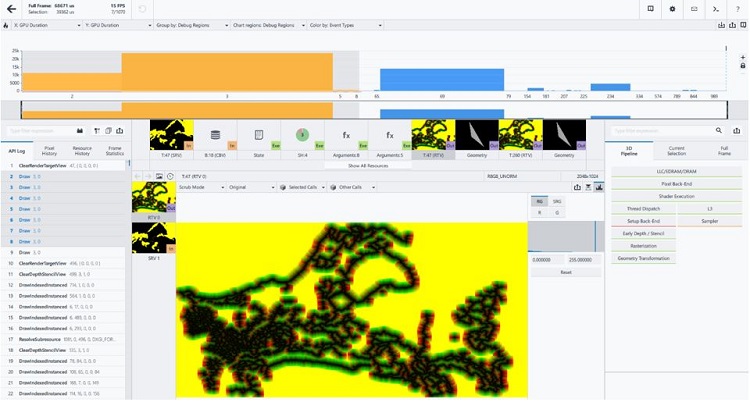
Figure 6. A long frame captured with the Intel® GPA tool. Orange boxes show the additional drawcalls that are not present in fast frames. Executing them takes almost 40 ms on an integrated GPU.
Technical Background
Before we move forward, I would like to introduce a couple of technical terms and algorithms that will be used later in the article.
Distance Field
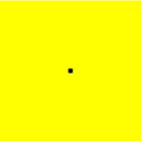
Distance Field is an interesting technique that utilizes a texture as a tool to describe complex shapes. You can think of such texture as a grid where, instead of color, each pixel holds the distance to the nearest geometry. Imagine borders between countries as the geometry—if we knew distances to that geometry for each pixel, we would be able to achieve a nice gradient around it, and this is exactly what Paradox did in Imperator: Rome.
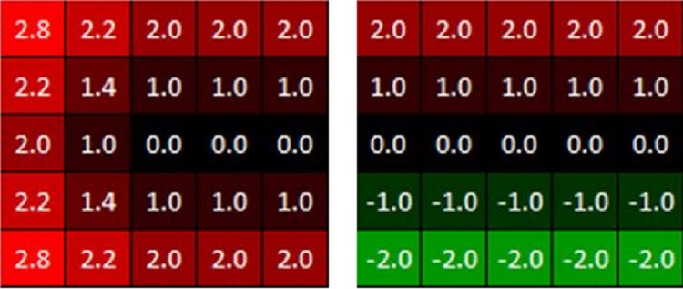
Figure 7. Examples of a Distance Field texture (sometimes referred to as “map”). The left one represents the Unsigned Distance Field, while the right represents the Signed Distance Field. Note that values 0.0 (representing the shape) are here for educational purposes only. In the actual texture there is no need to be this explicit.
In Figure 7 you can see two very simple 5x5 Distance Field textures. On the left the image represents an Unsigned Distance Field while the right image represents a Signed Distance Field—the sign tells us if the pixel lies inside or outside the geometry. Since the shapes we are trying to describe (the borders) don’t have an “inside” we can never have negative values, therefore we will be using Unsigned Distance Fields only. This also means our level of precision very close to the edges will be quite low: Paradox asks artists to be careful when tweaking the parameters for the mask to avoid artifacts around the edges.
Distance Fields have several advantages over keeping the map as an ordinary texture. First, the map is very big and keeping a single value instead of three (one for each color) significantly reduces the cost of sampling as well as the texture size itself. Additionally, Distance Fields help to maintain higher quality than an ordinary texture when you are close to the line —you could use this 5x5 texture to render into a 1080p render target and get a thin crisp line, whereas if you used a traditional texture it would be magnified and blurry. Lastly, the game allows modding which means that players and creators must be able to modify the map easily.
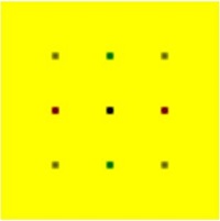
Jump Flooding Algorithm
The second important term is Jump Flooding Algorithm (JFA). In Imperator: Rome JFA is used to construct the Distance Field texture, but it has other applications, for example to construct Voronoi diagrams. The input to this algorithm is a texture that contains some arbitrary values that mean “no data”, which provide the seed for the JFA. In the case of Imperator: Rome these seeds would indicate borders in the game world. The algorithm then traverses this entire texture a couple of times and calculates the Distance Field for each pixel. It does so by sampling 8 neighboring pixels (4 in cardinal and 4 in ordinal direction) that are in a “step” distance offset from the given pixel. This “step” changes for each algorithm iteration. With information from all 8 pixels it determines the temporary closest distance to the nearest border.
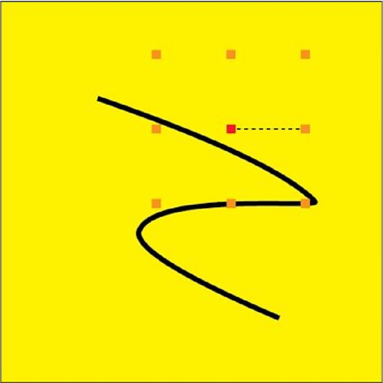
Figure 8. Jump Flooding Algorithm, distance calculation for one iteration of a single pixel.
Figure 8 should help with visualizing the algorithm. The red dot is a pixel for which we will be calculating the distance. Orange dots represent eight sampling points. The black line is a seed, or in other words the geometry, or the edge. This represents the actual border between the territories in Imperator: Rome. The dotted line represents a step which changes to a lower value for every iteration. Note that for this particular pixel the result would be incorrect since there is a closer geometry. However, this would be fixed in the further iterations where each step would be significantly lower.
Gradient Borders
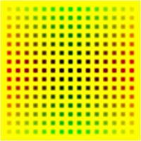
In Imperator: Rome borders between countries are shown as an overlay of the terrain, with a black spline to show the shape of the border and a color gradient to associate each side of the border with a country or other data, depending on the map mode. In this article I will only talk about the color gradient. Figure 9 is an example of how borders look in the game. The color gradient is achieved with two independent steps: a color lookup in a Color Map, and a sample from Distance Field texture.
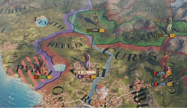
Figure 9. A screenshot from the gameplay, showing the application of a Primary and a Secondary Color. The border on Nepete territory uses red as primary color indicating that this is where the Rome border ends. Purple is the primary color for Pyrgi indicating ownership of the territory, and red is a secondary color, indicating that Rome currently occupies it.
Color Lookup
There are three different colors that a shader can access:
- Primary: the color you’ll see the most. Used as the primary color value of a map mode, for instance to show the owning country’s color in the default map mode (in Figure 9, the red color at the borders of Nepete or Carsioli territory)
- Secondary: this color is blended with the diagonal stripe pattern. Used for secondary color value of a map mode, for instance to show an invading country’s color as stripes over the owning country’s color in the default map mode (in Figure 9, the red stripes over Pyrgi)
- Highlight: used to highlight a province or area for the player by blending a color over it (rarely used, not shown in the picture)
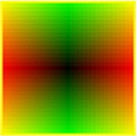
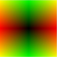
We hold all this information in a texture called the Color Map. The Color Map is recalculated whenever something relevant in the game state changes, like a province changing ownership, another country starting to occupy a territory, or when a player changes a map mode (as shown in Figure 10). The layout in which the Color Map holds the colors can be seen on Figure 11 on the right. The red rectangle indicates where the Primary color is stored, green rectangle indicates Secondary color and blue rectangle indicates Highlight color.
Figure 10. Whenever map mode changes, the Color Map is filled with new data.
We can obtain the color to use for any point on the map with one level of indirection. First, for each object that wants to use it (like terrain or mountains), we normalize the point coordinate from world-space to the 0-1 range in a pixel shader. Then we use that to point sample a huge lookup texture (8192x4096, R8G8_UNORM, Figure 11 on the left), which will give us UV-coordinates that we can use to get the primary color value from a much smaller Color Map (256x256, R8G8B8A8_UNORM, Figure 11 on the right). We can obtain Secondary and Highlight colors by simply offsetting those coordinates.
Figure 11. Color Lookup Texture (left) and Color Map (right). The Color Lookup Texture contains UV coordinates to use in the Color Map in order to obtain a Primary (red rectangle), Secondary (green rectangle) or Highlight (blue rectangle) color.
There is a reason for this indirection—the Lookup Texture needs to be calculated only once when the game starts and only needs two channels for the UV coordinates. This texture never changes afterwards. We need to calculate this instead of loading from it as predefined asset because scripts and mods can change how provinces are laid out. Then, when a color needs to be updated, we only need to update this single Color Map instead of what would be 3 uncompressed 8192x4096 4-channel textures.
Distance Field Texture
The second piece of information we need is how much blending of a color to apply, and for that we need a Distance Field Texture.
The Distance Field part is quite simple—as with the color lookup texture, we sample it using a normalized world-space coordinate. The coordinate normalization takes place in the pixel shader for all terrain, and the Distance Field Texture is sampled multiple times to make gradients a bit smoother. Each pixel in the Distance Field Texture contains an approximate distance to the “edge”. We use this value, combined with some constants and artist adjustable parameters, to calculate how much of the color we want to blend into the terrain.
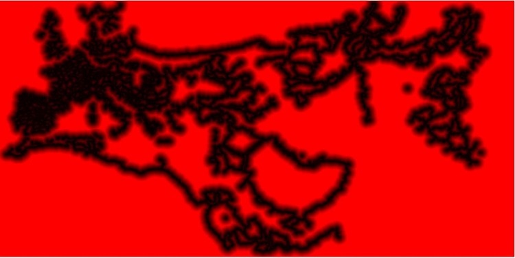
Figure 12. Final Distance Field Texture. Each pixel holds the distance to the nearest border.
Drawing Borders
Once we’ve applied the artist-provided parameters to the distance we’ve sampled from the Distance Field we get the Mask Value. This Mask Value can then be used to blend the color we get from the color map step into the terrain. Figure 13 shows all the pieces in one picture.
Distance Fields are effective because a low-resolution image will give almost as accurate results as a high-resolution image when sampled with a linear filter. The Gradient Borders system uses an Unsigned Distance Field which will have some problems with the precision close to the edges. Signed Distance Fields don’t have that problem. If you’re unfamiliar with signed distance fields I’d recommend reading Improved Alpha-Tested Magnification for Vector Textures and Special Effects by Chris Green of Valve*.
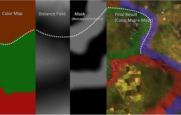
Figure 13. All the necessary components to calculate gradient for terrains. The Mask is the result of the application of artist-adjustable parameters to the Distance Field values. Color Map in this case is combined result of sampling both textures from figure 11. The white dotted line is a markup of where approximately the border lies.
Calculating Distance Field
The question that remains is how to create the Distance Field. We want to achieve a result where each pixel in the Distance Field texture contains the accurate distance to the closest edge. In practice we can’t get the exact results, but we can come pretty close—and quite quickly too.
The Distance Field is calculated on the GPU using a Jump Flooding Algorithm. Basically, what this means is that we first need to find the edges, and once we’ve found them, we can run JFA and “spread” the knowledge about those edges to neighboring pixels in (O(log(n)) iterations, where n is the maximum distance of the spread.
Running JFA on the GPU typically requires at least two-pixel buffers that are both read from and written to in a ping-pong manner – you read from one texture and write to another, then you swap the two textures, so that during the next iteration we read the results from the previous iteration and write to the input of the next iteration. In our Gradient Borders system these two textures use the R8G8_UNORM format. The two channels are used during the JFA to store distances to the closest edge in both axes separately, which allows us to use Euclidean distance metrics for good precision. We also have an R8_UNORM texture in which we store the final normalized distance (figure 12).
To sum it up before we go into detail, the Distance Field calculation executes four different steps.
- Pre-Pass for Coastal Border, which creates a mask used to suspend the creation of coastal borders in ocean provinces.
- The Init Step, which ensures that each pixel (in the down-sampled texture used to seed the JFA) contains either (255, 255) if all of the sampled pixels belong to the same “area-that-we-want-borders-around” or (distance-x, distance-y) if multiple areas are found within the sampled space; during this step we will sample the Color Lookup and Color Map a lot.
- Actual JFA algorithm performed in five iterations.
- The Distance Field texture creation from the JFA output.
Below is a table with snapshots for each step of that process. Each picture presents a 64x64 texture. The dot (which consist of four pixels) in the Init phase represents a seed for JFE. In-game, that dot would be replaced by country borders.
 |
Init. To seed the JFA we need to provide it with some initial data that it can expand on. To create this data we run one pass that will both detect the edges using the color sampling method mentioned earlier, and down-sample from the lookup texture’s size by a factor of 4 (a cheaper sample and distance field is a good way to compress distances since it can represent data in between 3 pixels). The 4 center pixels are not black but contain distances in x and y to the closest-pixel-of-another-color. The yellow pixels have the value (255,255) which means that the closest edge to this pixel is currently as far away as it can be. |
 |
JFA 1. In the first iteration each pixel will sample their neighbors with an offset of 16 pixels. A pixel will update its own value if the distance to the neighbor + the length of the vector stored in that neighbor is less than the length of the vector stored in the pixel. If updated the pixel’s new value will be the neighbor’s value plus the offset used to reach that neighbor. |
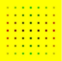 |
JFA 2. Repeat the previous step, but with an offset 8. |
 |
JFA 3. Same, but with offset 4. |
 |
JFA 4. Same with offset 2. |
 |
JFA 5. Finally, same with offset 1. It can be hard to see the differences between this and the previous step. Note that in the center of the Init step there is actually a 2x2 area that is initialized. If you look closely at the texture in the previous step, you’ll see that, while there are no gaps, every other pixel will “overshoot” and is not very precise. Now each pixel contains two values representing the distance to the closest edge in x-axis and y-axis, which can be treated as vectors. |
 |
The last step is where we create the gradient texture. All we need to do is to calculate the length of those two vectors for each pixel and we are done. |
To make things a bit more complicated, this is of course not enough to satisfy Paradox’s artists. The method described above, where we detect edges between provinces of different color, will work perfectly fine for most of the map. However, we will also get the gradients blending in on Imperator: Rome’s beautiful coastlines, which does not look very good. We tried simply ignoring edges towards water in the edge detection pass but that instead caused problems where two countries are divided by a large river for instance.
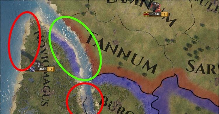
Figure 14. In green: Areas where we want gradients. In red: Areas where we don’t.
The solution was a pre-pass that supersamples the colors and creates a mask that tells the edge detection which parts of the map to ignore. It searches for specific “wildcard” colors and sets the mask to ignore edges for any pixel that is a wildcard and has only 1 or 0 nearby non-wildcard colors.
Below is an animated GIF that shows how distance information is populated for each step of the JFA for the entire map. And this is what was causing the performance stuttering—a big and complex simulation, running on a GPU with a lot of sampling from a very big texture.
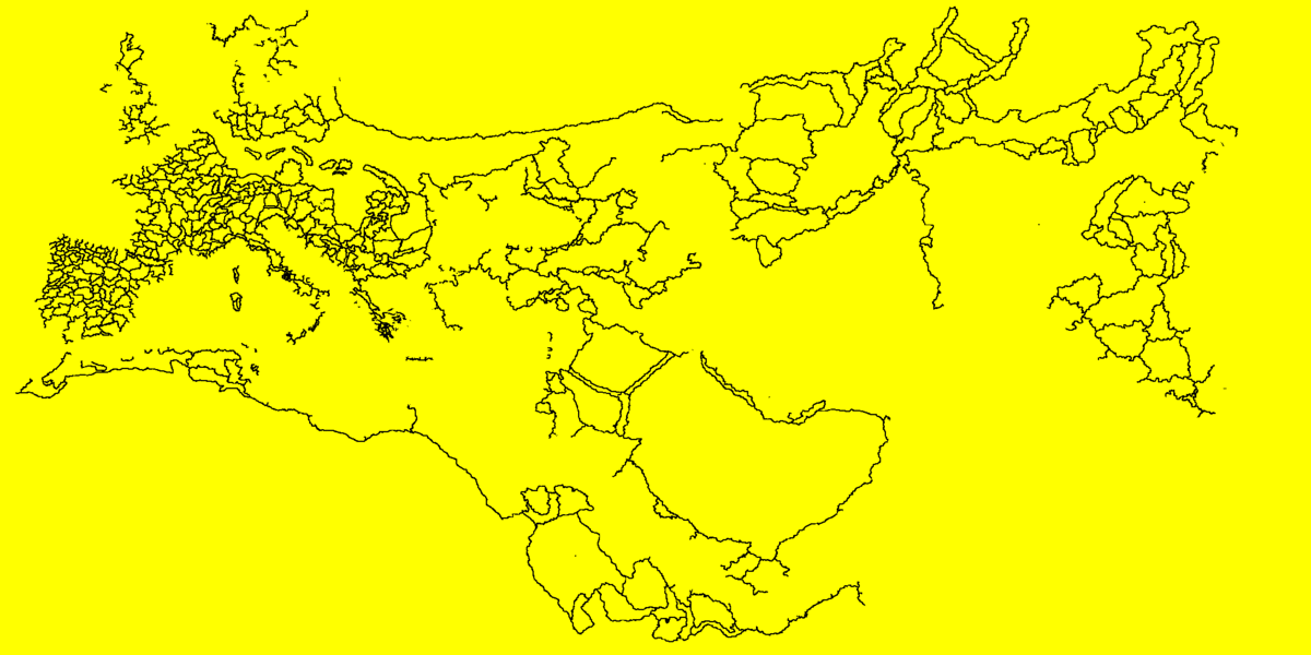
Figure 15. Animated process of Distance Field calculation for the entire map.
System Optimizations
The performance hit when calculating the gradients wasn’t very noticeable on the discrete GPUs. We could see a spike of a few milliseconds whenever the gradients were recalculated, but these events were rare and only an immediate result of the player pressing a button. We never profiled this feature on an integrated GPU where the spikes became very noticeable and irritating. Lesson learned.
The first thing that showed when we started profiling the issue was that these recalculation events weren’t as rare as we initially thought. It turned out that the gradients were being updated as soon as one of the three colors for a province was updated, even though the gradients only rely on one of those three. In addition, we never checked if anything had actually changed before recalculating the gradients. With those two issues fixed, we reduced the frequency of the spikes a lot, from one spike almost every in-game day to maybe one spike per month or so, if that.
But each spike is still very noticeable and irritating. After the first two fixes were implemented (only triggering for relevant color changes and making sure something actually changed before recalculating gradients) we could easily see and measure what parts of the map needed to be updated. Most of the time we only want to update a few provinces at once. Logs showed that we update either just a few provinces, or almost the entire map. There are some cases in between but those are very rare.
With this in mind, we decided that the most bang-for-buck optimization we could do was to optimize for the common case, which is a few provinces updating at a time. The entire gradient border update is done much like post effects: A very simple vertex shader for one single triangle that covers the entire clip space, and a pixel shader to do the actual work. The optimization we implemented switches the geometry from one “full-screen” triangle for the entire map to a list of quads where each quad covers an area in the distance field that needs to be updated. Simple, elegant, and very efficient. This optimization alone not only reduced the amount of work for the GPU but in turn also the number of samples, which was one of the main reasons for poor performance in this case. There were a lot of samples from a very big texture which caused inefficiency in caching and a necessity to fetch the data from system memory.
Generating the quads is also pretty straightforward. We already know the axis-aligned bounding box for each province, so all we need to do is to convert either the roof or the floor of that to a quad, but with some extra width so that the quad covers the maximum area that the gradient can affect. In other words, we extrude each side of the quad with the maximum distance of the distance field. When there are multiple areas that need to update there is a chance that the quads for those areas will overlap, which would mean a pixel could get calculated twice—and we don’t want that. To avoid the overlap issue, we let the CPU run the algorithm that cuts and merges the overlapping quads on a background thread before it is time to render. There is a tipping point where this quad-merging task start to cost more time than it saves (and the tipping point is different on different hardware), so keeping in mind that we want to optimize for the common case (where only 1-10 provinces are updated) we revert to updating the entire map when the number of quads needed gets large enough.
In Figure 16 you can see the quads that were generated after a country of about 6 provinces was annexed by the player. Since we know that nothing outside this area has changed, we can run JFA on this small area only instead of the entire map. Pixels near the edges of the quads can safely sample the pixels outside of the area and still produce the same result.

Figure 16. After the optimization, only a part of the Distance Field texture needs to be updated. Quads represents the area that needs to be updated after a country of 6 provinces is annexed by the player.
Conclusion
As you can see, performance is not always a matter of being either CPU- or GPU-bound—I would rather think of it as a measure of player satisfaction. Thanks to the great work of Paradox developers, the stuttering issue was addressed and fixed, and now more people can enjoy the game without any stuttering.
Last but not least, I would like to thank Daniel Eriksson from Paradox Development Studio for co-authoring this article, and Marcus Beausang (also from Paradox Development Studio) for reviewing it and helping with final touches. From the Intel side, I would like to thank Adam Lake for his extensive review. I did have to do a lot to re-work, but it was totally worth it, and the article is in much better shape than it initially was.
Tools and References
Get Windows Assessment and Deployment Kit (Windows ADK)
Get PresentMon*, a free tool that helps with performance measurements.
"