ISO3DFD Code Walkthrough

This tutorial with code examples is an Intel® oneAPI DPC++ Compiler implementation of a three-dimensional finite-difference stencil that solves the 3D acoustic isotropic wave-equation. This sample builds upon the concepts shown in the ISO2DFD Compiler Example.

Requirements

C++ programming experience and familiarity with the SYCL basics are assumed. If you do not have prior exposure with SYCL, read the SYCL resources listed at the end of this tutorial. For this tutorial, it’s recommended to first be familiar with the ISO2DFD equation and code walk through.

Introduction

This tutorial demonstrates solving a Partial Differential Equation (PDE) using a 16^th order finite-difference stencil for the 3D isotropic wave equation. The code is available on GitHub. This accompanying tutorial is intended as a deeper dive into optimizations you can do with SYCL.

Problem Statement

In the ISO2DFD code walkthrough we solved the wave equation for an acoustic medium with constant density, meaning there were only two spatial dimensions, X and Y. A more realistic situation can be seen in a 3D simulation in which we model sound waves traveling through air or water. In these situations, there are 3 dimensions, X, Y, and Z. In the equations below, the 2D case is on the left, and the right shows the equation for a 3D model.

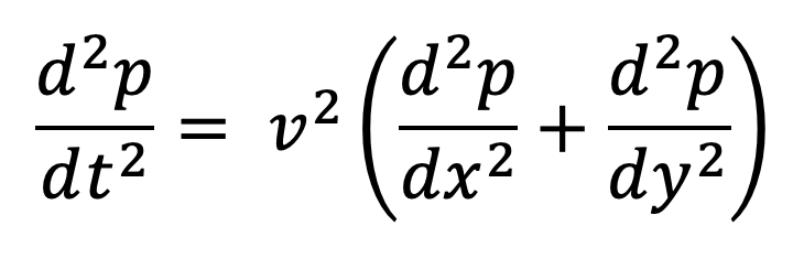
In these equations, p is pressure, v is the velocity at which the acoustic waves propagate in the medium, and t is time.

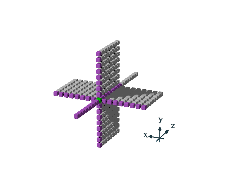
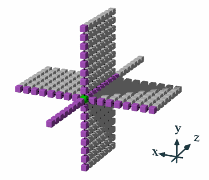
Since we’re solving for a 16^th order finite-difference stencil, that means for each point we calculate, we use the adjacent 8 values in each direction of the X, Y, and Z axis. This could be visualized like this:

The expanded equation looks like this, where the array C, holds the coefficients which are already adjusted by the changes in X, Y and Z.

Code Walk Through

Let’s jump right into the code walkthrough and we’ll see the optimizations in real time, as we learn about how they work.

Variables

To start, we parse the inputs. Depending on if you’re running the OpenMP or SYCL variant, the inputs could indicate different things. In this code walkthrough, we’re following the path of the SYCL implementation and will explore the optimizations for Shared Local Memory (SLM) as well. Thus, b1 and b2 inputs are the work group sizes used in the XY dimension, and b3 is the size of the slice of work in the Z dimension. Slicing in the Z-dimension allows auto-scalability i.e. an opportunity to scale-up or scale-down the total number of work-items which can be carefully chosen based on the number of execution units available on the GPU.

Usage: src/iso3dfd.exe n1 n2 n3 b1 b2 b3 Iterations [omp|sycl] [gpu|cpu]

n1 n2 n3 : Grid dimensions for the stencil

b1 b2 b3 OR : cache block sizes for cpu openmp version.

b1 b2 : Thread block sizes in X and Y dimension for SYCL version.

and b3 : size of slice of work in Z dimension for SYCL version.

Iterations : No. of timesteps.

[omp|sycl] : Optional: Run the OpenMP or the SYCL variant. Default is to use both for validation

[gpu|cpu] : Optional: Device to run the SYCL version Default is to use the GPU if available, if not fallback to CPU

We initialize n1-n3 as grid dimensions based on the first three inputs, and the following 3 are assigned to n1_block, n2_block, and n3_block. Additionally, in this stage we apply the (constant) changes in X, Y, and Z to the values in the Coeff[] array.

try {

n1 = std::stoi(argv[1]) + (2 * kHalfLength);

n2 = std::stoi(argv[2]) + (2 * kHalfLength);

n3 = std::stoi(argv[3]) + (2 * kHalfLength);

n1_block = std::stoi(argv[4]);

n2_block = std::stoi(argv[5]);

n3_block = std::stoi(argv[6]);

num_iterations = std::stoi(argv[7]);

}

…

// Compute the total size of grid

size_t nsize = n1 * n2 * n3;

…

// Apply the DX DY and DZ to coefficients

coeff[0] = (3.0f * coeff[0]) / (dxyz * dxyz);

for (int i = 1; i <= kHalfLength; i++) {

coeff[i] = coeff[i] / (dxyz * dxyz);

}

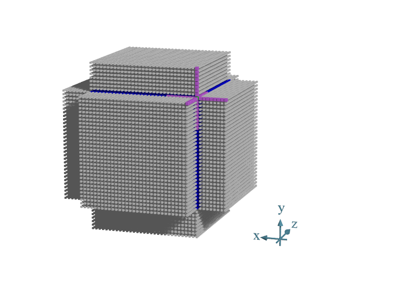
It’s important to note that the values n1, n2, and n3 have the addition of 2*kHalfLength. This is because the grid size represents the entire block, including the halo which is used for calculating edge points. Since for calculating each point, we require 8 extra points in all dimensions, the halo is used to add padding so no out of bounds errors occur.

In the image below, the point we’re calculating is in the upper right corner. The points needed for this calculation (8 in every direction, plus the previous value at that point), are colored purple. The grid is dark blue, and the gray points represent the halo of the grid. As you can see, when calculating any point near the edge of the grid, it’s necessary to use halo points.

Buffers

In the Iso3dfdDevice() function, we perform 3D wave propagation on the selected SYCL device. First, we create SYCL buffers which will be used as ping pong buffers to achieve accelerated wave propagation. We access these buffer elements with the next, prev, vel, and coeff parameters which are called in each loop iteration. SYCL buffers, accessors, and the concept of alternating between the next and prev parameters to save memory resources is described in the ISO2DFD code walk through. In this article, we’re focusing on the further optimizations to the ISO3DFD code, for a refresher on those concepts, read our ISO2DFD walk through.

// Create buffers using DPC++ class buffer

buffer b_ptr_next(ptr_next, range(grid_size));

buffer b_ptr_prev(ptr_prev, range(grid_size));

buffer b_ptr_vel(ptr_vel, range(grid_size));

buffer b_ptr_coeff(ptr_coeff, range(kHalfLength + 1));

As described in the ISO2DFD code walk-through, we alternate between next and prev parameters with each loop iteration, to effectively swap content each iteration in order to save memory resources. I refer to that as ping-pong buffers throughout this article.

The swapping of pointers occurs in the for loop which iterates over nIterations.

// Iterate over time steps

for (auto i = 0; i < nIterations; i += 1) {

...

#ifdef USE_SHARED

// Using 3D-stencil kernel with Shared Local Memory (SLM)

auto local_range = range((n1_block + (2 * kHalfLength) + kPad) *

(n2_block + (2 * kHalfLength)));

// Create an accessor for SLM buffer

accessor<float, 1, access::mode::read_write, access::target::local> tab(

local_range, h);

if (i % 2 == 0)

h.parallel_for(

nd_range(global_nd_range, local_nd_range), [=](auto it) {

Iso3dfdIterationSLM(it, next.get_pointer(), prev.get_pointer(),

vel.get_pointer(), coeff.get_pointer(),

tab.get_pointer(), nx, nxy, bx, by,

n3_block, end_z);

});

else

h.parallel_for(

nd_range(global_nd_range, local_nd_range), [=](auto it) {

Iso3dfdIterationSLM(it, prev.get_pointer(), next.get_pointer(),

vel.get_pointer(), coeff.get_pointer(),

tab.get_pointer(), nx, nxy, bx, by,

n3_block, end_z);

});

#else

// Use Global Memory version of the 3D-Stencil kernel.

// This code path is enabled by default

if (i % 2 == 0)

h.parallel_for(

nd_range(global_nd_range, local_nd_range), [=](auto it) {

Iso3dfdIterationGlobal(it, next.get_pointer(),

prev.get_pointer(), vel.get_pointer(),

coeff.get_pointer(), nx, nxy, bx, by,

n3_block, end_z);

});

else

h.parallel_for(

nd_range(global_nd_range, local_nd_range), [=](auto it) {

Iso3dfdIterationGlobal(it, prev.get_pointer(),

next.get_pointer(), vel.get_pointer(),

coeff.get_pointer(), nx, nxy, bx, by,

n3_block, end_z);

});

#endif

});

}

In this for loop, ifdef USE_SHARED is true if Shared Local Memory (SLM) was selected at compile time. By default, SLM is false, and the default code path is to use the Global Memory version of the 3D stencil. In the latter part of this code walk through, we cover the SLM optimizations.

The function Iso3dfdIterationGlobal() refers to the SYCL implementation for a single iteration of the ISO3DFD kernel. The image below shows how the stencil moves through the Z axis.

In this image we show, for each point we calculate, we use values 8 in each direction to calculate the new point value. The front[] and back[] arrays hold the values on the Z axis. Referring back to the equation for 3D wave propagation above, through will be stored in the front array, and through will be stored in the back array. These arrays are temporarily used to ensure grid values in the Z dimension are read only once then shifted in the array and re-used before being discarded.

float front[kHalfLength + 1];

float back[kHalfLength];

float c[kHalfLength + 1];

for (auto iter = 0; iter <= kHalfLength; iter++) {

front[iter] = prev[gid + iter * nxy];

}

c[0] = coeff[0];

for (auto iter = 1; iter <= kHalfLength; iter++) {

c[iter] = coeff[iter];

back[iter - 1] = prev[gid - iter * nxy];

}

With each iteration, only one new point will need to be read in from memory each time.

// Input data in front and back are shifted to discard the

// oldest value and read one new value.

for (auto iter = kHalfLength - 1; iter > 0; iter--) {

back[iter] = back[iter - 1];

}

back[0] = front[0];

for (auto iter = 0; iter < kHalfLength; iter++) {

front[iter] = front[iter + 1];

}

// Only one new data-point read from global memory

// in z-dimension (depth)

front[kHalfLength] = prev[gid + kHalfLength * nxy];

Additionally, as the 3D cube of values are stored in memory, an offset is used for indexing values in the X and Y directions. The Z direction is stored in order. Thus, when accessing the next element from memory, it is indexed very quickly.

Calculating the New Value

From here, we get into the main math calculations for each point. We calculate the first point, then enter into a for loop that updates the front and back arrays as described above and calculates the rest of the points in each Z plane.

With each iteration, we start with setting value to c[0]*front[0]. That meaning, value is the result of multiplying the previous value at that point by the first coefficient value. Then, we loop through kHalfLength times (8 in this case). With each iteration, we use the values at +iter and -iter in each direction from the value being calculated. front[iter] and back[iter] represent the Z direction. For the other two directions we must use the offset, gid and gid*nx to access the correct values from memory.

// Stencil code to update grid point at position given by global id (gid)

float value = c[0] * front[0];

#pragma unroll(kHalfLength)

for (auto iter = 1; iter <= kHalfLength; iter++) {

value += c[iter] * (front[iter] + back[iter - 1] + prev[gid + iter] +

prev[gid - iter] + prev[gid + iter * nx] +

prev[gid - iter * nx]);

}

next[gid] = 2.0f * front[0] - next[gid] + value * vel[gid];

gid += nxy;

begin_z++;

Once the for loop is completed and value has been fully calculated, we assign that value (with some additional math) to next[gid] and increment the gid and begin_z variables.

#pragma unroll(kHalfLength) is an optimization done to the code to improve instruction level parallelism.

Review

This section optimized memory lookups in the Z direction, but it leaves something to be desired in the X and Y directions since it’s looking up each value from memory with each call. In the next section, we take a look at the Shared Local Memory (SLM) optimizations. We’ll see how it compare to this SYCL implementation, and what improvements were made.

Shared Local Memory

Additional code has been added to this sample to show optimizations to use for Shared Local Memory (SLM). Directions for recompiling to enable SLM can be found in the README file:

// cmake -DSHARED_KERNEL=1 ..

// make -j`nproc`

The code for the SLM stencil is similar, and the calculation being done is the same, just this time we’re optimizing the X and Y dimensions in addition to the Z dimension. To visualize SLM optimizations, we take a look at a single Z-slice of the cube which is defined by parameters n1_block and n2_block.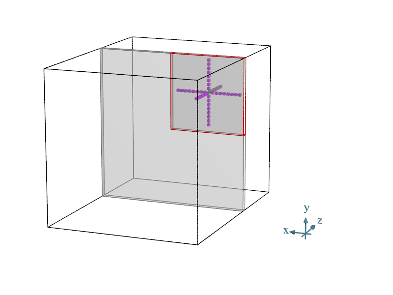

In the calculation, neighbors in the depth (Z-dimension) are read out of front and back arrays, same as before. Horizontal and vertical neighbors (X and Y dimensions), which are in the same work group, are read from the SLM buffers. Work groups and work items, as defined by DPC++, in addition with Z-slices used in ISO3DFD calculations are used to compute values in an organized and predicable way which allows maximum reuse of data.

Code Walkthrough

We start by defining the SLM buffer and accompanying accessor, called tab. From function Iso3dfdDevice(), we again use ping pong buffers, the only change is the function being called. Where Iso3dfdIterationGlobal() was called, now Iso3dfdIterationSLM() is called – with the exact same inputs.

From Iso3dfdIterationSLM(), we create work groups from each Z-slice of the cube, and work items from batches of global memory fetched and stored now locally. We perform all the calculations of that work group in a batch, in order to maximize memory reuse.

To start, we set up the begin_z, end_z, front, back, and c arrays. This is all done similarly as in the Global Stencil code. The interesting part begins when we get to the for loop where we iterate through Z slices.

for (auto i = begin_z; i < end_z; i++) {

...

// DPC++ Basic synchronization (barrier function)

it.barrier(access::fence_space::local_space);

// Only one new data-point read from global memory

// in z-dimension (depth)

front[kHalfLength] = prev[gid + kHalfLength * nxy];

// Stencil code to update grid point at position given by global id (gid)

float value = c[0] * front[0];

#pragma unroll(kHalfLength)

for (auto iter = 1; iter <= kHalfLength; iter++) {

value += c[iter] *

(front[iter] + back[iter - 1] + tab[identifiant + iter] +

tab[identifiant - iter] + tab[identifiant + iter * stride] +

tab[identifiant - iter * stride]);

}

next[gid] = 2.0f * front[0] - next[gid] + value * vel[gid];

// Update the gid to advance in the z-dimension

gid += nxy;

// Input data in front and back are shifted to discard the

// oldest value and read one new value.

for (auto iter = kHalfLength - 1; iter > 0; iter--) {

back[iter] = back[iter - 1];

}

back[0] = front[0];

for (auto iter = 0; iter < kHalfLength; iter++) {

front[iter] = front[iter + 1];

}

it.barrier(access::fence_space::local_space);

}

For each iteration, a forced synchronization occurs within the workgroup using barrier functions to ensure all the work items have completed while reading into the SLM buffer.

The bulk of the math calculations are nearly identical to the Global definition, with the only exception being that tab[] is used to call values in the X and Y directions, rather than calling from prev[] which referred to global memory. The neighbors in the Z-direction are read from front and back arrays, exactly the same as before. Now, neighbors in the X and Y dimensions are read from SLM buffers.

Tab Buffer

But what is tab and how does it work? tab is the memory buffer for Shared Local Memory, or scratch-memory. tab stores the data used for computing all the items within a workgroup. This can be visualized as below. The following diagrams demonstrate this for a halflength of 4, rather than 8. The workgroup (the points being calculated) is shown in blue. The tab buffer will hold all the points in the 16x16 area shown.

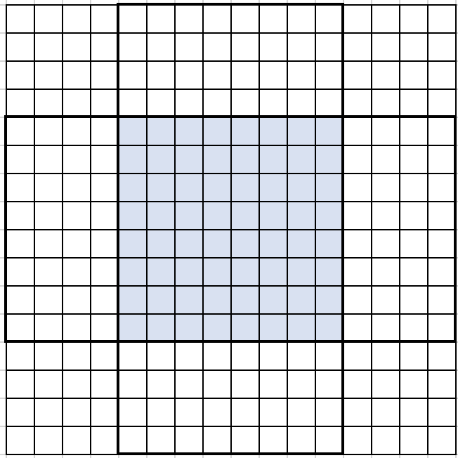
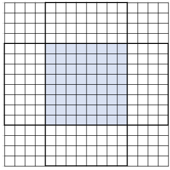
The halo points are outlined above, below, left, and right of the blue workgroup points. Before we begin any calculations, we must populate tab with those points, and the previous values of each work item. This is done in three steps.

First, we populate the upper and lower halo. By using an offset, each row of the workgroup within copy_halo_y will bring in an associated row of the upper and lower halo. Since GPUs process commands in parallel, it won’t necessarily be done in order, but it could be visualized as such:

This is done in the code:

if (copy_halo_y) {

tab[identifiant - kHalfLength * stride] = prev[gid - kHalfLength * nx];

tab[identifiant + items_y * stride] = prev[gid + items_y * nx];

}

Similarly, copy_halo_x populates the halo points to the left and right of the workgroup.

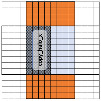
This is done when copy_halo_x is true in the code,

if (copy_halo_x) {

tab[identifiant - kHalfLength] = prev[gid - kHalfLength];

tab[identifiant + items_x] = prev[gid + items_x];

}

The final step is to populate tab with the previous values of each of the work items (all the blue points). This is done simply with,

tab[identifiant] = front[0];

Now, with tab populated, all work-items in the workgroup can read data from the SLM buffer, resulting in data-reuse for the X and Y directions out of SLM with expected lower latency and higher bandwidth. For the Z direction, front and back arrays are used, just like described before. So, when calculating each point for Shared Local Memory, only one call to global memory is necessary, that is the addition of one point each time the front or back array needs to be updated.

Summary

In this code walk through, we saw a few of the key optimizations done in the Iso3dfd code. We built upon concepts introduced in the ISO2DFD walkthrough and in this walkthrough introduced the concept of Shared Local Memory, which optimizes memory reuse for the X-Y direction.

These optimizations, though complex, demonstrate the capabilities of C++ with SYCL programming against various hardware targets. For more SYCL examples, check out our GitHub, or follow our getting started guide on the Intel Developer Zone.

Please note that the shared local memory (SLM) optimization explained above might not result in an efficiency improvement if the code is run on an Intel® Gen9 GPU, but it might show improvement on Intel® Gen12LP GPUs.

In both GPUs, SLM is a 128 KB highly banked data structure that is accessible to each of the 16 EUs in the subslice. The proximity to the EUs provides low latency and higher efficiency since SLM traffic does not interfere with L3/memory access through the dataport or sampler. 

Some architectural differences in Gen12LP, including improvements to the banking implementation to reduce hot-spotting and bank conflicts which results in overall improvement in efficiency of the SLM usage, might provide higher efficiency when using SLM optimizations.

Resources

Intel oneAPI

Explore SYCL Samples

Source Code