Introduction
Inverse kinematics (IK) technology was launched in the robotics field and studied to calculate joint angles to move robot arms (end effectors) to the target position with specific degrees of freedom (Figure 1). IK uses kinematic equations to determine the joint angles so that the end effector moves to a desired position. IK technology is now applied to many other areas such as engineering, computer graphics, and video games.
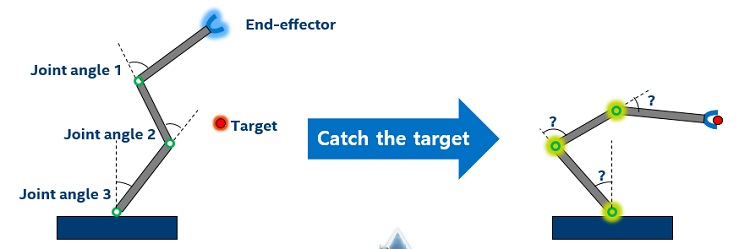
Figure 1. An example of inverse kinematics. The left robot arm has three joint angles, one end effector, and the target object. The right robot arm must determine the joint angles to move the end effector to the target object.
In 3D animation, there are generally two methods to animate a skeletal mesh. One way is to use forward kinematics, which feed direct rotational data straight into the bones of the skeletal mesh. It moves joints or bones directly according to rotation data. The second way is to use IK, which works in the opposite direction and gives a target position to the bone chain. An IK algorithm called IK Solver then calculates rotational data with which the end position of the bone chain (end effector) can reach the target position. When the target position changes, the IK Solver recalculates the rotational data and rotates the bones so the end effector meets the new target position.
IK animation makes character motions appear more natural and reactive in a game environment. For example, it can be used to keep a character’s feet planted on uneven ground or on stairs. It can also be used for a character’s hand hold on moving objects.
There are two traditional IK solutions. The analytical approach finds a single solution by using a closed equation, and difficult to formulate a closed form in the case of three or more links (Figure 2). The numerical approach finds solutions by iteratively using an error function until the error becomes minimized (Figure 3).
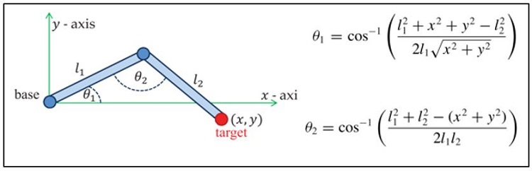
Figure 2. Analytical approach of IK solution. θ1 and θ2 can be calculated with a closed equation.
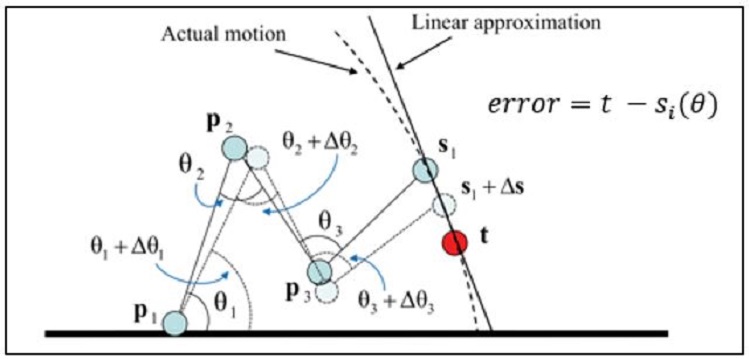
Figure 3. Numerical approach of IK solution. θ1, θ2, and θ3 are found using an error function.
When compared, these approaches have pros and cons. The numerical approach delivers better IK quality over the analytical approach, but it requires more computation time than the analytical approach. Although both approaches have advantages, they cannot provide high quality and large-scale IK simultaneously in a PC environment. This is because the high-quality IK solution requires a complex computation and significant computing resources so it’s difficult to support large-scale IK in a PC environment. In massively multiplayer online role-playing game (MMORPG)-style applications where many 3D characters must be animated, we need another approach to support high-quality IK animation in a PC environment (Figure 4).
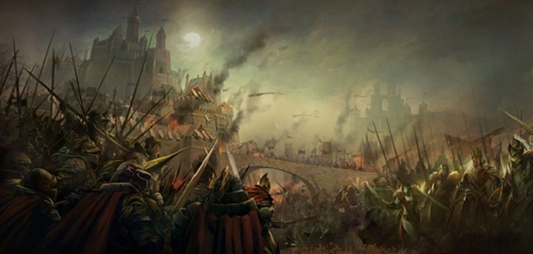
Figure 4. An illustration of siege warfare from NCSOFT*. In MMORPG-style game applications, many 3D characters need to be animated.
Recent research shows that deep learning and neural networks are useful tools for character control and human movements1, 2, 3. We are introducing a new approach to large-scale IK solutions. In this article, we consider full-body IK usage in MMORPG, where 100 characters must be animated, and each character has four end effectors and 23 joints (Figure 5). The full-body IK applies an IK Solver, not to a certain chain but to the entire armature.
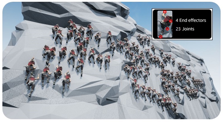
Figure 5. Demo screenshot of full-body IK animation for 100 characters ascending an uneven cliff. Each character has four end effectors (two hands and two feet) and 23 joints.
To solve the IK problem for large-scale character animation, we use two deep neural networks (DNNs). After describing the architecture of the two DNNs, this article discusses the optimization methods required to meet the product level of quality and performance. For performance optimizations, we only consider game applications on PC client environments, where both the graphic rendering and DNN inference tasks co-exist. First, we compare CPU against GPU when processing DNN inference tasks and game-play workload simultaneously. Next, we compare performance among various DNN libraries such as NumPy*, TensorFlow*, Intel® Math Kernel Library for Deep Neural Networks (Intel® MKL-DNN), and the Intel® Distribution of OpenVINO™ toolkit4. Finally, we describe how to change the workflow for batch processing and its effect on performance.
For the project described in this article, NCSOFT* took the lead role, which included ideation, DNN model design, and test app development. Intel had the supporting role, which included testing, optimization with the Intel Distribution of OpenVINO toolkit, and performance analysis.
Architecture of Deep Learning-based IK Solver
Our IK Solver is mainly composed of two DNNs. As input, it gets position data of current hands (two end effectors), current feet (two end effectors), next target hands (two target positions), and next target feet (two target positions). As output, it generates 60-frame motion data of character animation for two seconds (Figure 6).
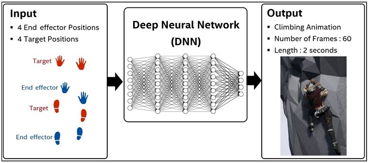
Figure 6. Architecture overview. LEFT: The IK Solver gets four current positions and four next target positions as an input. CENTER: The input data goes through the IK Solver, composed of two DNNs. RIGHT: The IK Solver generates 60-frame motion data of character animation for two seconds as an output.
We initially used a single DNN to generate motions, but it became very large in order to simultaneously infer and generate all the motions. The output result was not satisfactory. Also, there was significant computation cost and the output motions were low quality. We therefore spread the workload across two DNNs.
The first DNN creates the trajectory data of the animation (five points for a character’s movement path). The second DNN creates the pose data of the animation (23 joint rotation values of bones). Between the two DNNs, we use a Curve Fitting step to smoothen the trajectory data (Figure 7).
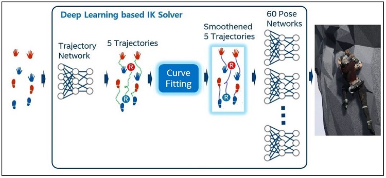
Figure 7. Architecture detail. The first DNN creates the trajectory data of the animation, and the second DNN creates the pose data of the animation. Between the two DNNs, the Curve Fitting step smoothens the trajectory data.
As the first step, input data is sent to the Trajectory DNN, and it generates trajectories of root and four end effectors (two hands and two feet). A trajectory is composed of 60 consecutive position data that corresponds to 60 frames of individual motion. Generally, there is some noise in DNN output and the noise tends to increaser for small-sized DNN. The output from Trajectory DNN also has some noise that causes trembling motions. We minimize the noise using the Cubic Hermite Spline5 Curve Fitting solution as the second step. As the last step, for each 60-motion frame, Pose DNN receives the root and four end effector positions that are smoothed through the Curve Fitting step, and it generates 23 joint angles, which constitutes one pose. From an architecture point of view, we made two key contributions. First, we divided a single large DNN into two lightweight DNNs to greatly improve performance. Next, we added a Curve Fitting step to improve IK quality by reducing noise in trajectories.
Training Data
In general, DNNs can execute an inference task with high-quality output only after they are trained with a very large amount of high-quality training data. In our project, almost 10,000 high-quality motion data are used for training the Trajectory and Pose DNNs. Because it’s almost impossible to get that amount of motion data from motion-capture devices directly, we generate motion data using the Jacobian method6, which is a numerical approach (Figure 8).
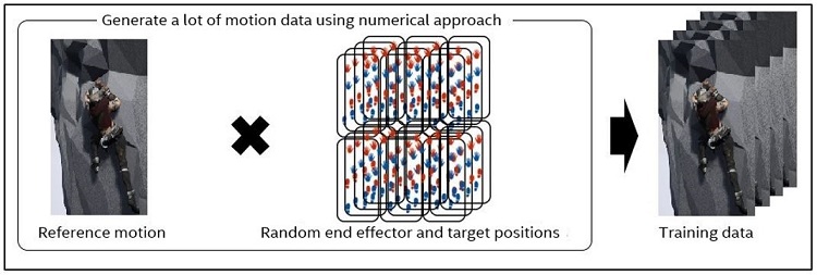
Figure 8. Training data generation. First, the reference motions are created manually. Next, the end effectors and target positions are randomized based on the reference motion. Finally, the additional motion data are generated using a numerical approach.
To generate the training data, we manually create one reference motion in the preferred style. We then randomize 10,000 position sets based on the reference motion (each set is composed of four end effectors and four target positions). Finally, we combine one reference motion with each position set and generate motion data using the numerical approach.
We can now train two DNNs on a dedicated server with deep learning frameworks, such as TensorFlow, using the 10,000 motion data. After the DNNs are trained, we can deploy them on game clients. Our IK Solver will execute inference tasks on the game clients after the deployment.
IK Quality Comparison
This section compares the animation quality of our IK Solver to a typical two-bone IK solution result from Unreal Engine* samples. Applying the same trajectory data, we see a more natural movement in our IK Solver at several body joints (Figure 9).
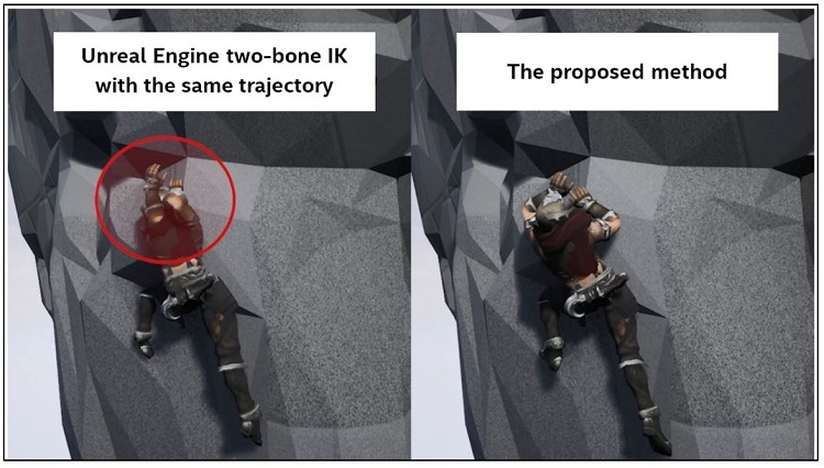
Figure 9. Quality comparison. LEFT: The character animation uses two-bone IK. RIGHT: Our full-body IK Solver is used for the character animation and shows more natural movement.
In Figure 9, the left-side character is gathering his arms unnaturally. While two-bone IK is likely to generate unintended motions, our full-body IK Solver generates more natural motions, as show on the right.
Optimization: CPU Versus GPU
This section describes general workload characteristics of game applications and our IK Solver’s inference tasks. Generally, game applications require low latency, as quick response is the critical factor to a positive user experience in games. Any kind of game lag usually breaks the user experience. For games that aim to achieve high-end graphics quality, the GPU resource is usually busy performing graphics-rendering tasks, while the multicore CPU resource has relatively more headroom (except for core 0, which hosts the render thread).
Regarding the workload characteristics of our IK Solver’s inference task, it uses very small neural networks and small batch sizes. The inference task needs to be performed for each game character using IK animation during each game loop iteration. Apart from the absolute hardware performance, the workload itself is rather friendly to current CPU architectures that can execute a small-sized inference task very frequently.
Considering workload characteristics of general games’ play and the IK Solver’s inference task, we can assume that using the CPU for processing the inference task is a better choice in terms of overall performance. To verify this assumption, we evaluate the overall performance of three commercial games’ play. We use the frame time (ms) and the number of inference tasks per second as performance metrics. We simply compare the performance metrics while playing three different commercial games where the CPU and GPU process the inference tasks. Note that this animation inference computation is not actually driving the animation of these tested games; rather, it is a proxy workload configuration to model how an inference computation might impact system performance. The runtime measurements were made using test machine A in Table 1.
Table 1. System configuration of test machine A.
| CPU | Intel® Core™ i7-6700K processor |
| GPU | GPU NVIDIA* GTX 1080 |
| Memory | 16 GB |
| OS | Microsoft Windows® 10 |
Before measuring the frame time of the games, we first check CPU and GPU utilization during major game play time (Figure 10).
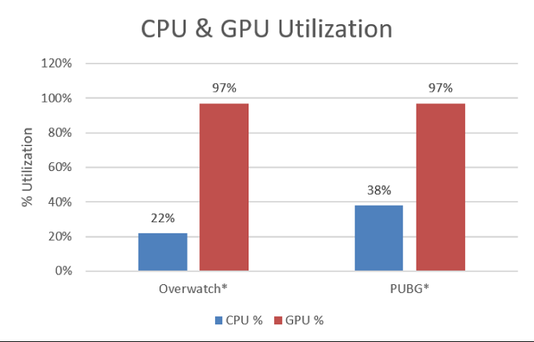
Figure 10. CPU and GPU utilization without IK inference task on test machine A.
Viewing the results, we see that the multicore CPU has more headroom, while most of the GPU resource is used during game play time.
To see more detail on how the added DNN inference tasks affect the game performance for the games, we first measured the game latency without DNN inference tasks as a baseline. Then, we measured the game latency while running TensorFlow-based inference tasks as a separate OS process on GPU and CPU, respectively (Figure 11). The game latency is the frame time during which one frame is processed.
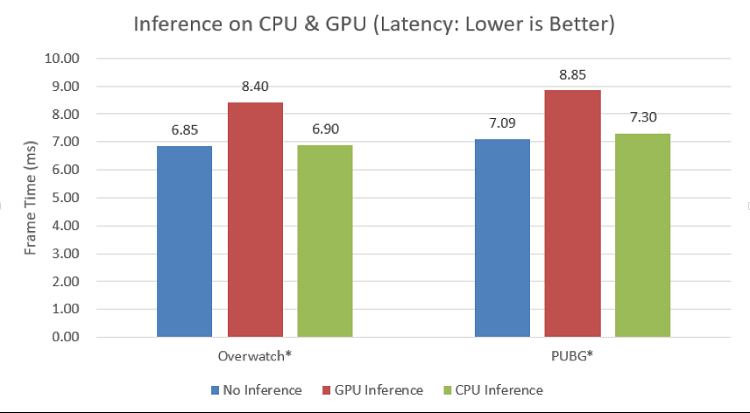
Figure 11. Latency change with IK inference tasks on test machine A. The blue bar shows the frame time without inference tasks, the red bar shows the frame time when the GPU processes the inference tasks, and the green bar shows the frame time when the CPU processes the inference tasks.
Viewing the results, processing the inference tasks on the CPU only slightly affects the frame time, while moving the inference workload onto the GPU noticeably increases the frame time.
We also measured the inference throughput on both the GPU and CPU while running the games (Figure 12). The inference throughput is the number of inference tasks processed during one second.
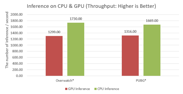
Figure 12. Inference throughput on GPU and CPU on test machine A. The red bar shows the number of inferences per one second that the GPU processes, and the green bar shows the number of inference per one second that the CPU processes.
Viewing the results, the inference throughput is higher on the CPU because processing inference tasks on GPU and playing the games compete with each other for the GPU resource. In this context, we choose the CPU for processing inference tasks and focus on CPU optimization for increasing the inference throughput.
Optimization: DNN Libraries
In this section, we measure the performance of different DNN libraries: Naïve C++ (OpenMP*), NumPy (OpenBLAS), TensorFlow (Eigen* 1.12.0), and the inference engine of the Intel Distribution of OpenVINO toolkit (2018 R5). All runtime measurements were made using test machine B in Table 2.
Table 2. System configuration of test machine B.
| CPU | Intel® Core™ i9-7900X processor |
| Memory | 16 GB |
| OS | Ubuntu* 16.04 LTS |
We take average response time (latency) as a performance metric for each library. To see the performance scaling, we measure the latency according to the core count (Figure 13). The latency is the processing time spent by all the inference tasks to create 100 IK motions.
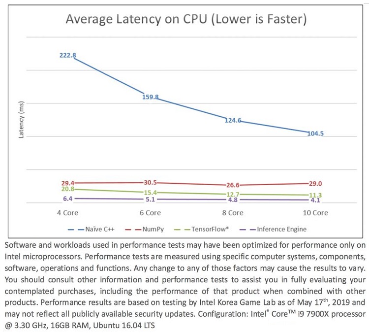
Figure 13. Average latency of DNN libraries on test machine B. The blue bar shows the latency that is the total processing time to complete the inference tasks by each library for the 4-core configuration. The red bar shows the latency for the 6-core configuration, the green bar shows the latency for the 8-core configuration, and the purple bar shows the latency for 10-core configuration.
As Figure 13 shows, the inference engine of the Intel Distribution of OpenVINO toolkit shows the best performance with the shortest latency.
Regarding the general workflow of a DNN model deployment to a game client, the model is first trained in the various environments. Then, the Model Optimizer converts the trained model into the Intermediate Representation (IR) format. Finally, the Inference Engine loads this IR and processes the inference tasks on the game client (Figure 14).
The free Intel Distribution of OpenVINO toolkit lets users optimize deep learning models for faster execution on Intel® processors. The toolkit imports trained models from Caffe*, Apache MXNet*, and TensorFlow, regardless of the hardware platforms used to train the models. Developers can quickly integrate various trained neural network models with application logic using a unified application programming interface. The toolkit maximizes inference performance by reducing the solution’s overall footprint and optimizing performance for the chosen Intel® architecture-based hardware.
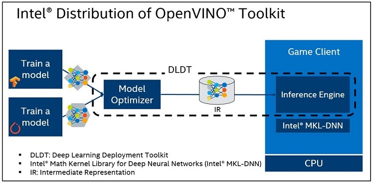
Figure 14. The Intel® Distribution of OpenVINO™ toolkit incorporates the Deep Learning Deployment Toolkit (DLDT). The DLDT is mainly composed of the Model Optimizer and the Inference Engine.
After running Intel® VTune™ Amplifier, we can see that Naïve C++ has the OpenMP library, NumPy has the OpenBLAS library, TensorFlow has the Eigen library, and the Inference Engine has the Intel MKL-DNN library as one of the hotspot functions (Figure 15).

Figure 15. Top five hotspot functions for the Naïve C++ version, the NumPy version, the TensorFlow version, and the Inference Engine version.
Optimization: Batch Processing
If we process the same operation multiple times, it becomes obvious that we can improve the throughput by uniformly grouping multiple operations and process once in a batch. For example, if there are four fully-connected layers with three inputs and three outputs, they can be processed in a batch as each instance has the same shape (Figure 16).
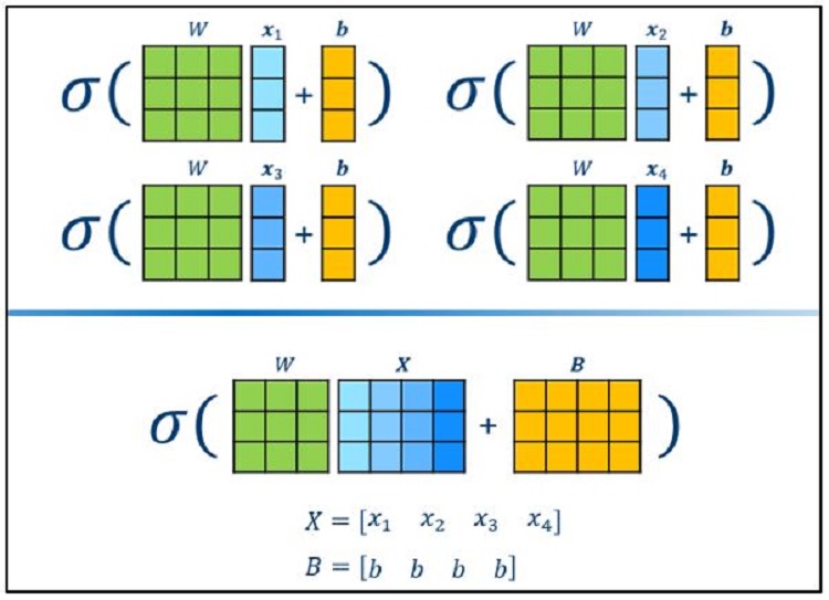
Figure 16. Batch processing example. It generally shows better throughput to group multiple operations in a uniform way and process once in a batch.
This section describes how we changed the workflow for batch processing to improve throughput efficiently. The early IK Solver couldn’t process a character’s request in batches. In game applications, there are multiple characters that request the IK Solver to generate IK animation pose data. For every game loop, each animating character makes the request for the next frame. Because it is time-consuming work for the IK Solver to process each request one by one, we added the Batch Manager to efficiently collect and manage requests for the IK Solver (Figure 17).
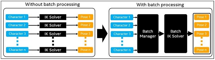
Figure 17. Workflow change in batch type. LEFT: Each character requests its dedicated IK Solver to generate IK animation pose data. RIGHT: All characters request one batch manager that processes the IK requests in a batch.
As described in section 2 of this article, our IK Solver consists of three major processing steps: Trajectory, Curve Fitting, and Pose. With the Batch Manager, Trajectory and Pose steps can work in batches. However, the Curve Fitting step couldn’t be executed in batches as it used the Cubic Hermite Spline algorithm in cubic polynomial form. Figure 18 defines the polynomial of the Cubic Hermite Spline.
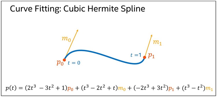
Figure 18. The polynomial of the Cubic Hermite Spline. The t can be substituted for any value between 0 and 1 to get a point on the curve.
Calculating p(t) is simple. However, because it needs 25,000 calculations to create motions for 100 characters, we need a more efficient calculation method. Generally, multiple polynomials can be expressed in one matrix form. For example, there can be one matrix combining six polynomials that solves six points for t0 to t5 (Figure 19).
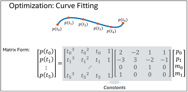
Figure 19. Multiple polynomials in a matrix form. One matrix can express six polynomials that solves from p(t0) to p(t5). As the value from t0 to t5 are constants, the gray-shaded parts also become a constant after one matrix multiplying in advance.
In this matrix form, the gray-shaded parts can be considered as a constant after one matrix multiplying in advance, and six points can be obtained by a single matrix multiplication at runtime. We can, therefore, run the Curve Fitting step in batches like Trajectory and Pose steps (Figure 20).
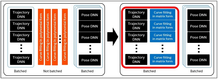
Figure 20. Curve Fitting in a batch type. LEFT: The Curve Fitting step uses the Cubic Hermite Spline algorithm that is in polynomial form. RIGHT: The algorithm is transformed to a matrix expression for batch processing.
We evaluate each transformation for the batch process to see how much it improves the performance (latency). The workload is to generate 100 characters’ worth of motion data for 60 frames (Figure 21).
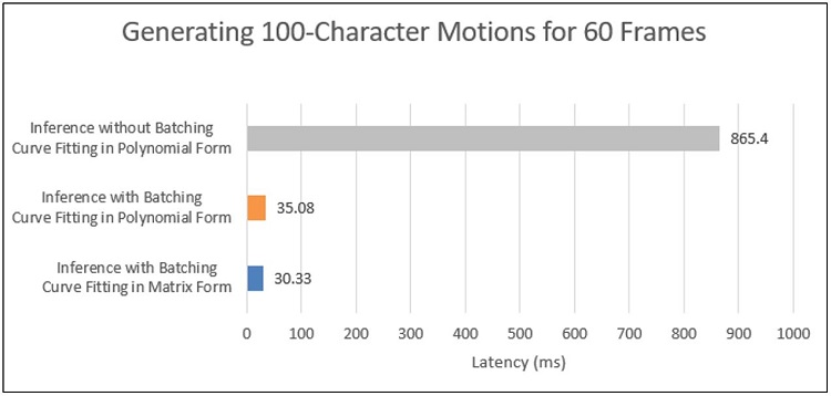
Figure 21. Latency for generating 100 characters’ motion data for 60 frames on test machine B. The gray bar shows the latency that is the total processing time to complete the inference tasks without batching and the Curve Fitting in polynomial form. The orange bar shows the latency by batching and the Curve Fitting in polynomial form. The blue bar shows the latency by batching and the Curve Fitting in matrix form.
In the first test, we computed the inference task one at a time without batching; the Curve Fitting was in polynomial form. It was extremely slow. For the second test, we computed the inference task with batching; the Curve Fitting was in polynomial form. The latency was drastically reduced. Finally, we transformed the polynomial form of the Curve Fitting step into a matrix form and processed all inference steps in batches. The latency was further reduced.
To convert the final result into a standard performance metric, Frame Time, we break down the final latency into average Trajectory and Curve Fitting time and average Pose time separately (Figure 22).
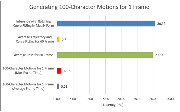
Figure 22. Frame time conversion of the latency for generating 100 characters’ motion data on test machine B. The blue bar shows the final latency by batching and the Curve Fitting in matrix form. The orange bar shows the time that Trajectory and Curve Fitting steps consume out of the final latency. The green bar shows the time that Pose step consumes out of the final latency. The red bar shows the maximum frame time. The purple bar shows the average frame time.
The Trajectory and Curve Fitting step is executed once for 60 frames, while the Pose step is executed once per frame. We calculate the maximum frame time by adding the Trajectory and Curve Fitting time to the Pose time per 1 frame (1.19 ms = 0.7 ms + (29.63 ms ÷ 60)). We calculate the average frame time by dividing the final latency by 60 (0.51 ms = 30.33 ms ÷ 60). The final result exceeds our expectations; we had targeted 5 ms as our goal.
Summary
We demonstrated how to generate the large scale of inverse kinematics motion data with a deep learning approach. We divided a single large DNN into two lightweight DNNs and used Curve Fitting processing to reduce noise out of the Trajectory DNN. Regarding performance optimization, we saw that processing the inference tasks on the CPU has little effect on overall game performance when compared to processing the same workload on the GPU. This is typically because the GPU is already overloaded to handle additional workloads, while multicore CPUs often have idle cores or threads. We then evaluated the performance of different DNN libraries. Finally, we showed how batch processing of inference tasks can improve performance.
Regarding the inference engine of the Intel Distribution of OpenVINO toolkit, we saw a performance benefit to processing inference tasks on the CPU. In the future, we may explore using Intel® Processor Graphics to process these workloads.
NCSOFT developed a simple demo game in which 100 game characters ascend a rugged cliff with the Unreal Engine* 4 and our IK Solver. We verified that each character moved both their hands and feet more precisely while touching the cliff’s surface. NCSOFT plans to deploy the IK Solver on their commercial game in the near future.
About the Authors
Intel
Tai Ha is a Senior Application Engineer at Intel with more than 10 years of experience in software development and 13 years in software optimization for datacenter, media, and game applications.
Kyle Park is a Senior Application Engineer at Intel who has worked more than 10 years on back-end servers in cloud services and 9 years on software optimization for AI, datacenter, High-performance computing (HPC), and game applications.
Jeff Park is a Senior Technical Consulting Engineer for Intel. He has worked on the optimization and debugging of Intel® systems and software for 6 years. Before that, he was an embedded software developer and system debug engineer for 14 years.
NCSOFT* AI Center, Game AI Lab
Dr. Hanyoung Jang is the Team Leader of the Motion AI team of NCSOFT, a global game company. He has researched in the fields of robotics, General-purpose computing on graphics processing units (GPGPU), computer graphics, and AI. Currently, his primary research interest lies in creating natural character animation through deep learning.
Hyoil Lee is a Team Leader of the AI System team of NCSOFT. After receiving his Master’s degree in Computer Science from Korea University in Seoul, he gained 10 years of experience in software development, embedded systems, and algorithm optimization. For the past three years, he has been designing and developing machine learning systems.
Dongwon Yoon is a Senior Game AI Researcher at NCSOFT. Dongwon has more than 10 years of experience, specializing in server engineering and service operation. Over the last few years, he has developed AI-related solutions with a focus on optimizing deep learning inference and the simulation of reinforcement learning systems.
Footnotes
1. Katerina Fragkiadaki, Sergey Levine, Panna Felsen, and Jitendra Malik. Recurrent Network Models for Human Dynamics. In Proceedings of the IEEE International Conference on Computer Vision, pp. 4346–4354, 2015.
2. Daniel Holden, Taku Komura, and Jun Saito. Phase-Functioned Neural Networks for Character Control. ACM Transactions on Graphics (TOG), 36(4):42, 2017.
3. Julieta Martinez, Michael J Black, and Javier Romero. On Human Motion Prediction Using Recurrent Neural Networks. arXiv preprint, arXiv:1705.02445, 2017.
4. Intel Distribution of OpenVINO™ toolkit
5. Gerald Farin. Curves and Surfaces for CAGD: A Practical Guide (5th edition). Morgan Kaufmann Publishers Inc., San Francisco, CA, USA, 2002.
6. Samuel R. Buss. Introduction to Inverse Kinematics with Jacobian Transpose, Pseudoinverse and Damped Least Squares Methods. IEEE Journal of Robotics and Automation, 17(1), 2004.